Learning about Empirical DSGE Analysis

Hey Community,

in the upcoming weeks I would like to invest my time to learn as much as I can about “empirical DSGEs”.

I know that there is already a lot of literature writen about the estimation of DSGE models and related empirical applications, e.g. Smets & Wouters (2003, 2007); An & Schorfheide (2007); the Handbook Chapters in the Handbook of Macroeconomics of Lindé et al. (2016) and Fernández-Villaverde et al. (2016) as well as the Chapter of Del Negro & Schorfheide (2013) in the Handbook of Economic Forecasting.

To understand this empirical literature I have to study a lot.
This brings me to the question of whether there is a path of least resistance?

What would be the necessary study plan to start with before I can replicate the first empirical paper?

I would like to focus on bayesian estimation of DSGE models in the first step.

Fortunately, I have a modest understanding of bayesian statistics as well as DSGE models, but ironically I have no clue when it comes to the combination of both.

It would be nice, if someone could outline a path of least resistance like a series of introductory material which introduces me into this field.

I would start with a textbook like https://web.sas.upenn.edu/schorf/companion-web-site-bayesian-estimation-of-dsge-models/

Hi Max1,

I can suggest you read


before reading Fernández-Villaverde et al. (2016) , which is a bit more technical :slight_smile:
1 Like

@jpfeifer and @cmarch: Thanks for the recommendations.

I already started reading the textbook of Herbst & Schorfheide.
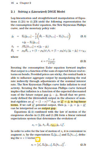
Is there any supplementary material in existence to facilitate the derivations of some of the equations in this textbook? I already noticed that there is an additional document with corrections.

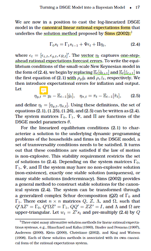
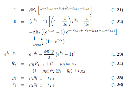
For example, I would like to know the exact formulas for the matrices in equation 2.4.

I also have a question whether there is a document with corrections for the Sims (2002) paper?

Since the textbook of Herbst & Schorfheide relies on the Sims (2002) solution method, I tried to cast the model mentioned there into the canonical form \Gamma_0 y_t = \Gamma_1y_{t-1} + C + \Psi z_t + \Pi \eta_t.
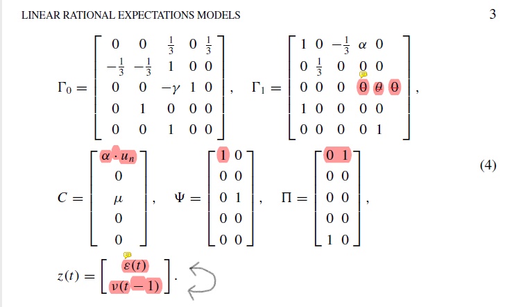
By doing so, I wasted some hours because the solutions for the matrices mentioned by Sims (2002) in equation (4) are wrong and the definition of \eta_t is missing.

  1. I don’t have the book with me. Could you post a photo of the equation.
  2. AFAIK, there is no correction available for the Sims-paper.
  1. I have attached the required screenshots of Herbst & Schorfheide.
    Pic3
  2. I will upload my solution for equation (4) in Sims (2002) by the end of today.
    It would be nice if someone could doublecheck it.

Here is my solution for the canonical form of the example model used by Sims (2002).
document.pdf (72.9 KB)

Here is a screenshot of the solution from Sims (2002) where I highlight the discrepancies between the solutions.


Pleas let me know, if you agree or disagree with my solution.
For me the definition of \eta_2(t) = E_t W(t+1) - E_{t-1}W(t+1) looks strange.

Here is my solution for the canonical form of the small-scale DSGE in Herbst&Schorfheide (2015) [equation (2.4)]
Herbst&Schorfheide eq. 2.4.pdf (81.3 KB)

Can somebody help me out with the derivation of equation (2.10) in Herbst & Schorfheide (2015)?

The question is:
How to cast the canonical form

\begin{align}\Gamma_0 s_t = \Gamma_1 s_{t-1}+\Psi \epsilon_t+\Pi\eta_t\end{align}

into the VAR(1) representation of the DSGE?

\begin{align}s_t = \Phi_1(\theta) s_{t-1}+\Phi_\epsilon(\theta) \epsilon_t\end{align}

I can follow the argumentation until we arrive at the point:
\begin{align}\begin{pmatrix}\Lambda_{11}&\Lambda_{12}\\0&\Lambda_{22}\end{pmatrix}\begin{pmatrix}w_{1,t}\\w_{2,t}\end{pmatrix} = \begin{pmatrix}\Omega_{11}&\Omega_{12}\\0&\Omega_{22}\end{pmatrix}\begin{pmatrix}w_{1,t-1}\\w_{2,t-1}\end{pmatrix}+\begin{pmatrix}Q_1\\Q_2\end{pmatrix}\left(\Psi \epsilon_t+\Pi\eta_t\right)\end{align}
where we apply generalized Schur.

Now, we should reorder the eigenvalues such that the lower subsystem depends on the instable eigenvalues. Overall stability requires that w_{2,t}=0 \forall t.
As far as I understand having a unique stabel solution is equivalent to w_{2,0}=0 and \eta_t = -{(Q_2\Pi)}^{-1}Q_2\Psi\epsilon_t.

Now we reach the point, where I got lost. I already looked up Lubik & Schorfheide (2003) and Sims (2002) to see it they can help me out, but his attempt was not successful.

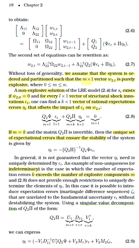
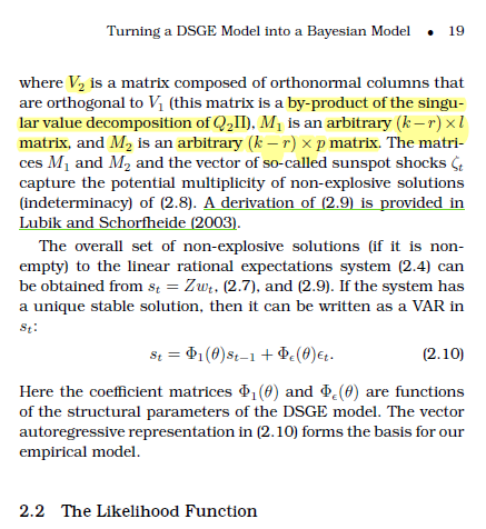
I am confused by the following sentence in Herbst&Schorfheide (2015, p.19):

The overall set of nonexplosive solutions (if it is nonempty) to the linear rational expectations system (2.4) can be obtained from s_t = Z w_t, (2.7), and (2.9). If the system has
a unique stable solution, then it can be written as a VAR in s_t:

If I think about this sentence, then I would expect that the sunspot shock \zeta_t shows up in the solution. But this is not the case in eq. (2.10).

Can I ignore this sentence and derive the VAR(1) representation by plugging
w_{2,t}=0 and \eta_t = -{(Q_2\Pi)}^{-1}Q_2\Psi\epsilon_t into the upper subsystem?

I attach two screenshots such that you know what I am talking about.

19 - Kopie

That implies the absence of sunspot shocks, because then the solution would not be unique anymore. A sunspot shock is not uniquely pinned down by the model.

Then my suspicion is true that the previous sentence has nothing to do with equation 2.10.

Unfortunately, the textbook is silent and gives no further hints w.r.t. eq. 2.10.

If I use the stability condition w_{2,t}=0\forall t and \eta_t=-{(Q_2\Pi)}^{-1}Q_2\Psi\epsilon_t and solve for the stable upper subsystem I end up with
\begin{align}w_{1,t}= \Lambda_{11}^{-1}\Omega_{11}w_{1,t-1}+\Lambda_{11}^{-1}Q_1(I_n-\Pi{(Q_2\Pi)}^{-1}Q_2)\Psi\epsilon_t\end{align}.

What remains to be done until we arrive at
\begin{align}s_t=\Phi_1(\theta)s_{t-1}+\Phi_\epsilon(\theta)\epsilon_t\end{align}?

Using Z_1s_t=w_{1,t} might be an option, but unfortunately Z_1 is not invertible.

I finally managed to derive the VAR(1) representation of the canonical form.
The solution approach is based on Sims (2002).
Herbst&Schorfheide eq. 2.10.pdf (99.0 KB)
Please let me know if I made a mistake.

What is missing is the exact formula for \Phi which satisfies the equality of
Q_{1\cdot}\Pi = \Phi Q_{2\cdot}\Pi.
I don’t think that Q_{2\cdot}\Pi will be invertible in general even if we have a unique stabel solution.
Or am I wrong?

In equation (49) the Sims (2002) paper suggests a solution.
Unfortunately, I am unfamiliar with the singular value decomposition.

The SVD should help you deal with cases where the matrix to be inverted is singular. Did you have a look at other textbooks like Dejong/Dave?

Do you mean this one? https://press.princeton.edu/books/hardcover/9780691152875/structural-macroeconometrics

Sims (2002, p.11) mentions a condition for the row space of Q_{1\cdot}\Pi and Q_{2\cdot}\Pi which must be satisfied, but in his paper he applies the SVD to the column space (see eq. 49 on page 13).

So he leaves it to the reader to make the necessary adjustments.
My guess is to simply transpose Q_{1\cdot}\Pi and Q_{2\cdot}\Pi and then apply the SVD.
But Herbst&Schorfheide don’t adjust the SVD this way as you can see above eq. 2.9.

Yes, that is the correct reference. Note the Errata at https://sites.google.com/site/pfeiferecon/teaching

1 Like