why does perfect foresight ramsey give me multiple solutions (depending on the starting guess) with this timing of the (cont. time) euler equation and definition of real rate:
(C(+1)-C)/(C*Deltat)= r-rho_hh_t;
r      = (R(+1)-delta*q(+1)+(q(+1)-q)/Deltat)/q;
but a unique solution with this timing:
(C(+1)-C)/(C*Deltat)= r(+1)-rho_hh_t;
r      = (R-delta*q+( q-q(-1))/Deltat)/q(-1);
Sorry for the delay. I figured that there is no multiplicity for the first timing (i just had a bug). However, the two timings of r do provide different solutions even though they should be isomorphic in my opinion.
I attach the file. in lines 52-62 you can choose between the two different timings (version 1 and version 2) by commenting/uncommenting the 4 relevant lines (i omitted 2 lines in my original question above).
For sure, if I specify a policy (pi=0) instead of using Ramsey, then the two timings deliver the same result.
Many thanks!
Maybe @MichelJuillard does know. There is a difference in the steady state for the Lagrange multipliers. It’s clear why the timing matters for stochastic models due to the presence of expectations. But there also seems to be a timing convention here for the perfect foresight approach. I am attaching a version with a macro processor directive for selecting the case. example.mod (5.5 KB)
My guess is that Dynare takes r at time t to be the variable controlled by the Ramsey planner.
I’m not entirely sure. The model is a bit too complex to follow easily what is going on. Ramsey policy optimize outcomes given the state of the economy before starting Ramsey policy. It is not immediately clear whether the state variables are the same in the two versions of the model. Check for a variable that would appear in t-1 in one version of the model, but not in the other.
sorry for the delay in the response. I hope you had a nice Christmas break!
@Michel, you said the model is a bit to complex. This is a standard NK model with capital and capital adjustment costs. But importantly, the only differences between the two model versions is how the real rate r is defined.
In version 1 r is defined as the expectation of next period marginal real return on capital. Hence wherever r is used it appears as r(0): in the Euler equation, Phillips curve and the capital pricing equation.
In version 2 r is defined as current marginal real return on capital. Hence wherever r is used it appears as r(0): in the Euler equation, Phillips curve and the capital pricing equation.
Thanks to both for pointing out the differences in the state variables.
However, I am having trouble to understand what dynare ramsey is doing here. In particular, I don’t understand,
Why ramsey is turning control variables (like C, Y, r or iota) into states, as Johannes said. In the screenshot below I did algebraically what I would expect dynare to do, and this doesn’t change the nature of variables.
Why ramsey delivers different solutions to 2 model versions which appear isomorphic to me.
Would you expect this behaviour of dynare ramsey? Can you explain it?
Is there a way to have a look at the equation system that ramsey solves? Something like dynamic_resid.m but where the variables and parameter names are still written out.
Many Thanks!
Dominik
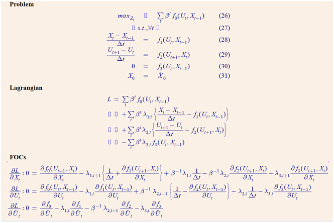
Attachment: Generic ramsey optimization problem in dynare notation.
X: Dynamic States
U: Dynamic Controls
Usquiggle= Static Controls
note: Usquiggle is missing in the functions f0, f1, f2, f3. That is a typo.
Thanks Johannes for the quick reply, this is helpful. It immediately answered question 1 (Because the equations in my code do have exactly the same form as the generic example). I’ll check if it also helps with the more tricky question 2.
Hi Johannes and Michel
I think the reason why optimal policy in the two models is different has to do with the information sets that are used on impact. I wonder if this behavior is desirable.
But let me go step by step.
1
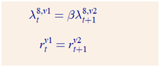
I looked at the equation systems that are solved, and if one ignores the information sets (which aren’t expicit in dynare language anyway), then the two models are isomorpic if one defines the following relationship between the model variables in the two versions (where lambda^8 is the planner’s 8th multiplier (MULT8) and v1 and v2 denotes the two versions). (1)
Note: The first line explains the difference in the SS values that Johannes noted above.
2
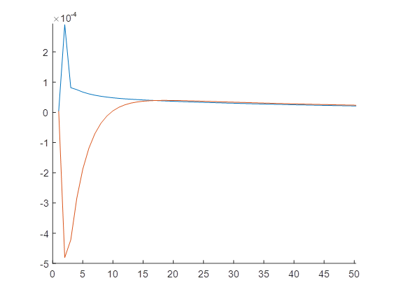
And indeed if I use the solution of model version 2, lag the paths of r and MULT8 in line with the above formula the residuals are 0 for all periods but the first.
3
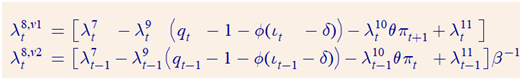
In order to understand why I checked the FOC of the planner wrt r. For the two versions, they are given by (2)
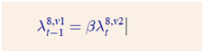
According to the relationship in (1) the 8th multiplier’s in the two versions should be related as follows for the two models to be identical: (3)
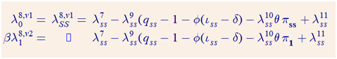
One can verify that this holds for all t>1. However, using the above definitions of lambda8 for t=1 and keeping in mind that t=0 is the SS we get: (4)
there is a difference between the two lines: pi_1 vs pi_SS.
This inconsistency would disappear if the FOC wrt r for version 2 (see equ. 2) would instead read (5)
where pi_t has been replaced by its expectation one period ahead.
4
I think it would be desiderable that the solution to model versions 1 and 2 were identical. My hunch is that the solution to version 1 is the correct solution. And ramsey could be djusted to deliver 5 for version 2, which would be identical.
Apologies for the last post being a bit long and messy, it took me a bit to get here. I attach a pdf file that compares the model versions 1 and 2 and shows how they lead to different solutions, which I believe to be undesirable. This document makes the same point as section 3 above, but is hopefully easier to follow. compare version 1 and 2.pdf (110.0 KB)
Conclusion:
I believe ramsey with perfect foresight may have a bug in how it treats information sets on impact. It assumes that E_{t-1}(x_t)=x_t. This is correct for t>1 (by perfect foresight) but not for t=1 (since the shock in t=1 is unexpected - “MIT shock”).
This problem is behind the finding that two isomorphic models (versions 1 and 2) deliver different results.
in Dynare, the information set is defined so that current shock is observed before taking decisions about t-period variables. This is also true for Ramsey policy computations.
I’m not sure how your last pdf relates to the beginning of the discussion. Here you compare two different models while the discussion started about what seemed to be two ways to write the same model. However for the reasons that I presented above, under Ramsey policy, in first period these two ways of writing the model don’t have the same implications.
Thank you very much for getting back. I apologize for not being clearer.
Throughout all my posts, including the pdf, I always refer to the same 2 model versions, which differ only in the timing of the way the return on capital is defined. I believe the two models to be isomorphic from a economic point of view. Yet they lead to different solutions when used with ramsey and perfect foresight.
It seems you agree that the 2 versions (without ramsey) are isomorphic. So what am I to make from the fact that ramsey optimal policy is different across the 2 versions?
I agree. The problem I am pointing at is that ramsey seems to assume E_0(x_1)=x_1 (where the shock occurs in t=1). So it appears to me as if ramsey mixes up period 1 decision variables and their 1 period ahead expectations - when the shock is not yet observed/expected and the economy is in the SS.
Furthermore I believe that this possible inconsistency is the reason why i dont get the same results for ramsey policy of two model versions, which i believe should deliver the same results.
For Ramsey problem, Dynare maximizes “welfare” in period 1, given the state of the system in period 0 and x_1 is observed before computing the optimal policy. As we are operating under perfect foresight conditional expectations don’t apply here. Agents and policy maker know all future shocks.
I don’t believe that the difference between the two representations under Ramsey comes from the fact that x_1 is observed, because it is the case in the two versions. What changes comes from the fact that the different timing used for interest rates/returns has an implication about the surprise of the private agent implied by the switch to optimal policy in period 1.
I tend to agree with @MichelJuillard that it’s not a bug, but the logic of the setup - which is tricky here. In case you define the expected the return to be forward-looking
\begin{eqnarray}
L & = & \sum_{t}\beta^{t}...\\
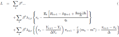
& & +\sum_{t}\beta^{t}{{\lambda_{1,t}}}\left\{ r_{t}-\frac{R_{t+1}-\delta q_{t+1}+\frac{q_{t+1}-q_{t}}{\Delta}}{q_{t}}\right\} \nonumber \\
& & +\sum_{t}\beta^{t}\lambda_{2,t}\left\{ \left(r_{t}-\frac{Y_{t+1}-Y_{t}}{\Delta Y_{t}}\right)\pi_{t+1}-\frac{\varepsilon}{\theta}\left(m_{t}-m^{\ast}\right)-\frac{\pi_{t+1}-\pi_{t}}{\Delta}\right\} \nonumber
\end{eqnarray}
the first constraint says that r_0, which is known at time 0 depends on the choices at time 1. But the Ramsey planner only starts choosing variables at time 1. Thus, r_0 is taken as fixed, because it was based on choices that were taken before the Ramsey planner was able to re-optimize. These ancient choices are now relevant for the second constraint. The fundamental point is the assumption that variables are part of the information set of their time period. So r_0 must be known at time 0. Due to reoptimization by the planner at time 1 it is not.
Things are different in the second setup
\begin{eqnarray}
L & = & \sum_{t}...\\
& & +\sum_{t}\beta^{t}{{\lambda_{1,t}}}\left\{ r_{t}-\frac{R_{t}-\delta q_{t}+\frac{q_{t}-q_{t-1}}{\Delta}}{q_{t-1}}\right\} \nonumber \\
& & +\sum_{t}\beta^{t}\lambda_{2,t}\left\{ \left(r_{t+1}-\frac{Y_{t+1}-Y_{t}}{\Delta Y_{t}}\right)\pi_{t+1}-\frac{\varepsilon}{\theta}\left(m_{t}-m^{\ast}\right)-\frac{\pi_{t+1}-\pi_{t}}{\Delta}\right\} \nonumber
\end{eqnarray}
because the use of r_{t+1} for the second constraint tells us that the current choices of the planner are important.
Regarding Johannes’ post, what you say indeed explains the difference in dynare solution between the two versions. And it also shows why I think it is a suboptimal timing convention.
In my opinion, the first constraint in the Lagrangian should be read as (I added the expectations, similarly I could add them in the second constraint)
Since E_0(x_1)~= x_1 (since the shock at t=1 is an MIT shock) the ancient value r_0 should hence not be relevant for the second constraint.
I am not sure I understand your point. Adding the expectations does not change anything here. Due to the break in behavior when the Ramsey planner starts, the expectations suddenly changes from time 0 to time 1. The time 0 expectations was taken with respect to the old regime while the time 1 expectations is taken with respect to the economy governed by the Ramsey planner.
Also, I don’t think there is any other good way to do this. Essentially you are arguing that we should simply plug in backwards from the dynamic equation in the first constraint. But by that logic, there is no first period where the Ramsey planner starts. You would be going back into the infinite past.
I have though about the problem again. My conclusion is that there is indeed nothing wrong with dynare. What I suggested above would not work. But when using ramsey users should be aware of the following rule, which may not be obvious to everyone (it could be added to the manual):
Avoid using forward-looking definitions as proper model equations / variables when using computing “timeless” ramsey policy (i.e. when the planner’s multipliers are not 0).
E.g. do not add the variable return to your model together with the below equation - you might wanna do so so to make the Euler equation easier to read, but don’t. Return=(Rental_rate_of_K(+1)+(1-delta)*q(+1))/q
However, you can introduce such definitions as model local variables. E.g.: #Return=(Rental_rate_of_K(+1)+(1-delta)*q(+1))/q
Introducing such definitions as proper variables with a proper equation may deliver incorrect optimal policy results. This is what happened to me in model versions 1 and 3 above.
Here is en explanation why this is happening. In short, introducing such auxiliary variables change the timing of the problem that ramsey solves, even though their introduction does not change the private equilibrium. explanation.pdf (77.0 KB)
 (1)
(1) (2)
(2) (3)
(3) (4)
(4)