Hello everybody!
For the purpose of the final paper I have to give back in order to complete my master in economics I decided to replicate the work of Lubik Schorfheide (2007) and model a small open DSGE economy (Canada) to analyse the decomposition of the shocks in the model.
The estimation of my parameters were tricky at first but with the help of this forum it seems to be holding nicely right now. I used bayesian estimation and recycled the posterior distribution obtained by Lubik and Schorfheide as my prior distribution. The results are plausible enough.
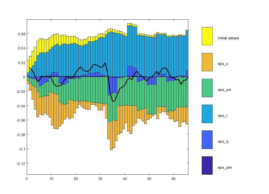
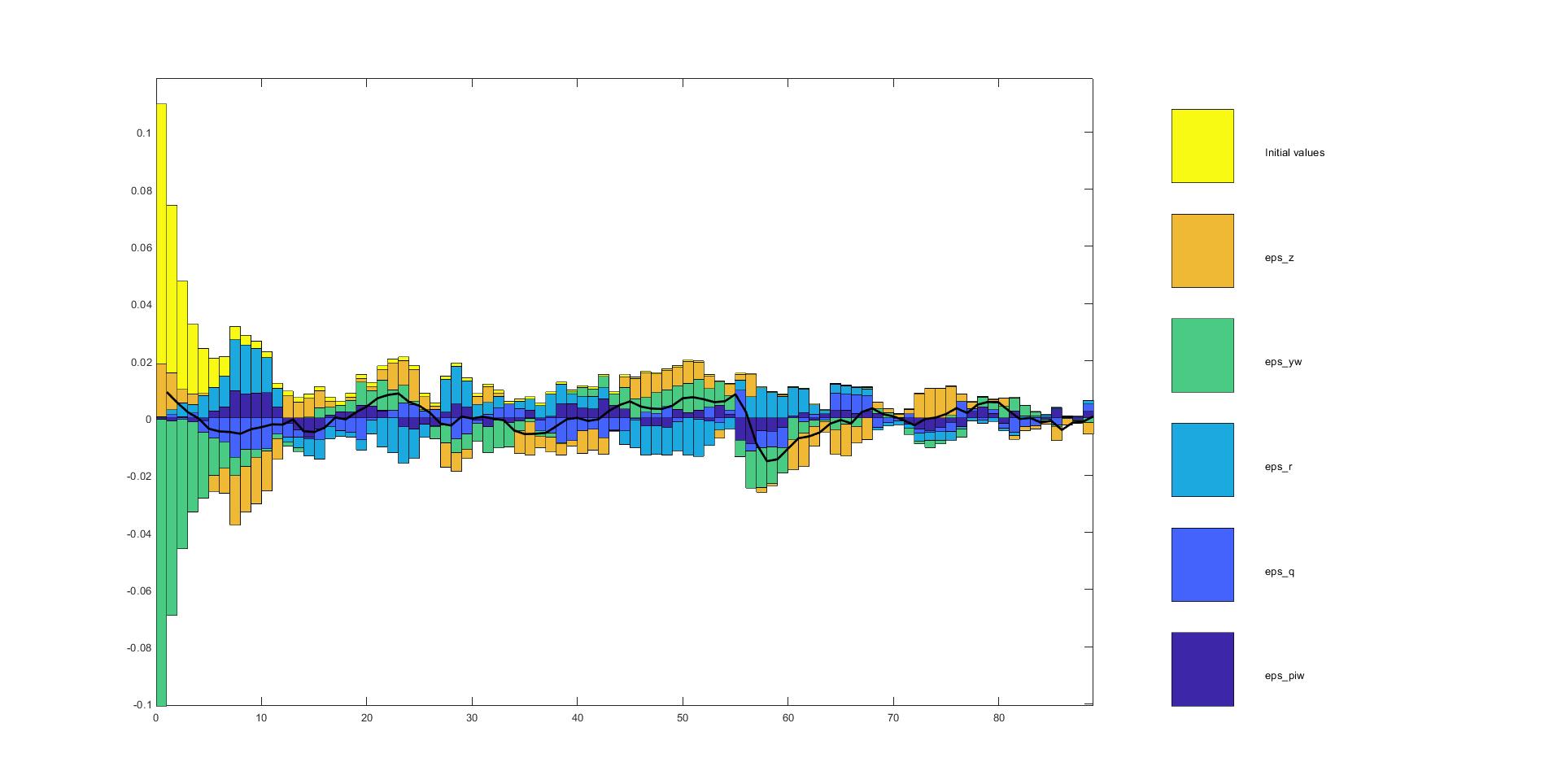
The next step was to decompose the shocks with the ‘‘shock_decomposition’’ command, which was, again, trickier than expected but I managed to get some plausible results. This post is about the intuition behind the results that I have obtained.
So here are my questions:
-
I’m having a hard time understanding how to analyse the shock decomposition that Dynare gives me back. I can’t wrap my head around how the shock related to technology growth (z) only pulls my y_gap downwards (represented as: actual output - potential output). A positive technology shock should have a positive influence on ‘‘y’’ (the output) which i turn would give me a positive result on y-yp, that is unless ‘‘yp’’ was subjected to the exact same influence (which is not the case).
-
I have tried many sets of different observed variables to feed to Dynare with many different results. Is there a rule of thumb to decide what variables to keep as observed variables? For the moment I tried to keep only the most crucial ones, and since I am limited to 5 (I have 5 shocks in the model) I am wondering which should be kept for good.
-
I used the real value of the exchange rate (CAD/USD) for the variable ‘‘e’’. At first I had log-linearized that value, then tought I could represent it as a trend value with the HP filter, then decided to go with the real value. Overall, I’d say I have no idea which would yield the most conclusive results. Everything else in my model is in it’s log-linearized version, so that would make sense to do the same for the exchange rate.
I think that’s all for now. You will find every necessary file to run the code in that post, feel free to use it for your own experiments/research.
Have a great day!
Alexis
I only have access to dynare 4.4.3 for now
lubikdecomp.txt (2.7 KB)
lubikdecomp.xlsx (30.7 KB)