How to simulate a cross section of firms

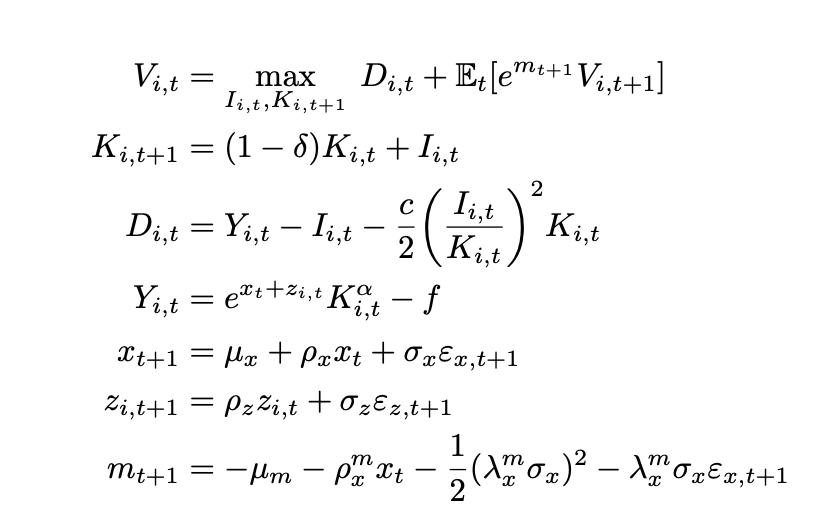
This is a simple neoclassical model of investment with a stochastic discount factor.

This model features an aggregate shock x_t and an idiosyncratic shock z_{i,t}.

When it comes to simulation, I want to simulate a cross section of firms, say 100 firms, that they share the same process of x_t but differ in their processes of z_{i,t}. In addition, all firms start ex ante identical, they have the same K_{i,0} and z_{i,0}.

Can you elaborate what you are trying to do? Is this a partial equilibrium setup? It looks like you could simply simulate one firm at a time given a fixed sequence for x_t but different shocks for z_{i,t}

1 Like

Hi Johannes,

Thank you so much for your prompt reply.

Yes this is a partial eq setup. It is really simple and nothing fancy here. My question is about generating the cross section.

I want to generate a cross section of firms to compare their valuations and expected returns.

Yes, your suggestion sounds right. How can I simulate the model for a fixed sequence of x? In particular, how can I integrate with matlab where I can write a loop to simulate the cross section and store simulation results?

FYI, I am new to Dynare…

Your first need a full description of the model, i.e. you need to derive the first order conditions describing the problem. Then you enter the model with the two shocks in Dynare. Simulating the cross-section can be done once the model works for one firm.

1 Like

Sure I can do finish the mod file. I will ask later about the simulation once the mod file is uploaded.

I have an additional question: in Dynare, is it possible to calculate V_t ? Can I simply put V_t = D_t + \mathbb{E}_t[ e^{m_{t+1}}V_{t+1} ] in the model section in mod file? Otherwise, how should I calculate V?

Yes,that recursive definition is the standard way of coding up value functions in equilibrium.

1 Like

toymodel.mod (1.4 KB)
toymodel.pdf (104.3 KB)

I provide the code as well as a draft of the toy model.

I am really struggling with the timing of variables. My understanding of the timing convention is that, upon observing the shocks at the beginning of period t, firms make optimal investment decisions.

That is why I try to use predetermined. However, it is still not what I expect due to the timing convention of Dynare…

In other words, investment decisions are made at the beginning of period t. As a result of the investment decisions, you obtain dividends, valuations. When it comes to the end of period t or the beginning of period t+1, the next-period dividend and valuation are realized, you have the realized return, as I write in the pdf file.

Can you help me here? I struggle all night but only get even more confused…

Let me try to be more explicit here.

What I don’t understand is that, in Dynare, the policy function is a function of both state variables and exogenous shocks. If one were to numerically solve the model using value function iteration, the policy function will be a function of state variables only, i.e., I_t = f(K_t, X_t, Z_t). That is, given the current level of K_t, X_t, Z_t, the firm chooses the level of investment I_t such that V_t is maximized in expectation.

Similarly, in consumption-based models, the household chooses the optimal consumption. For example, in long-run risk models, the consumption-to-wealth ratio is a function of expected growth and uncertainty.

In summary, there is no role for exogenous shocks in the policy function.

I dont know how to square that difference… I am truly confused here.

Use the attached file with Dynare 6.1. It obeys Dynare’s timing convention for exogenous states, which must be entered contemporaneously. Capital is declared as predetermined.
toymodel.mod (2.1 KB)

Regarding your question: yes, in global solutions only the exogenous state Z_t appears explicitly. But its persistence and therefore the states’ past values matter when discretizing the state space e.g. using Tauchen’s method. The points on the grid for the exogenous capture both the persistence and the shock value.

1 Like

Thank you so much for correcting my code and, in fact, rewriting a significant portion of it. I truly appreciate your help! I am able to run your file smoothly with Dynare 6.1.

I have some questions regarding the code and Dynare in general

  1. Why do you declare level variables instead of log variables? As I read from Dynare tutorials, both are fine and legit. And log variables provide an easier interpretation of IRF, no?

  2. What is the purpose of declaring var(log) y;? From what I read, y remains the level of output, not log output.

  3. Could you explain this line for SDF? What does “#” at the beginning represents? I understand that, because you specify m is driven by ex(+1), accordingly, you use m instead of m(+1) in the FOC.

#m = -rf - 0.5*(lambda_mx * sigma_x)^2 - lambda_mx * sigma_x * ex(+1);

[name='FOC']
1 + theta * i/k = exp(m) * (alpha * y(+1)/k(+1) + 0.5 * theta * (i(+1)/k(+1))^2 + (1-delta) * (1+theta * i(+1)/k(+1)));
  1. How can I set seeds in the simulation
N_firms=5;
N_periods=500;
x_rand=randn(N_periods,1);
z_idio=randn(N_periods,N_firms);
log_y_pos=strmatch('LOG_y',M_.endo_names,'exact')
log_y_save=NaN(N_periods,N_firms);

for iter=1:N_firms
ex_=NaN(N_periods,M_.exo_nbr);
ex_(:,strmatch('ex',M_.exo_names,'exact'))=x_rand; %keep fixed
ex_(:,strmatch('ez',M_.exo_names,'exact'))=z_idio(:,iter); %iterate over firms
y_=simult_(M_,options_,oo_.dr.ys,oo_.dr,ex_,options_.order);
log_y_save(:,iter)=y_(log_y_pos,2:end);
end
  1. Could I interpret the specification of the timing as follows:

At the beginning of period t, exogenous shocks \varepsilon_{x,t} and \varepsilon_{z,t} are realized.
The firm yield output Y_t = e^{x_t + z_t}K_t^{\alpha}, where K_t is the capital stock also at the beginning of period t.
Upon observing these shocks, the firm chooses the level of investment to maximize its firm value V_t.
The firm maximizes the cum-dividend value of the firm V_t, which equals the sum of current dividend D_t and the expected discounted value of the continuation value \mathbb{E}_t[M_{t+1}V_{t+1}], where M_{t+1} is driven by the shock \varepsilon_{x,t+1} realized in the beginning of the next period t+1.
The resulting V_t is realized at the end of period t after the investment decision is made.
Although we distinguish the beginning/end of the period t, they are all just labelled by time t.

  1. Could I calculate the value and return of the firm as follows? (Assuming that I have declared those variables)
[name='cum-dividend value']
vc = d + exp(m) * v(+1);
[name='ex-dividend value']
ve = exp(m) * v(+1);

Subsequently, I can calculate returns in matlab as follows

r = vc(2:end) ./ ve(1:end-1);
Regarding the policy function, I am still not sure that I understand it.

In the current version, the persistent of z is set to 0. In other words, shocks to z will not be incorporated in z and last for some periods. As a result, \varepsilon_{z,t} and will not enter the optimal investment policy function.

If I set the persistence to a positive number (say), then \varepsilon_{z,t} will show up in the policy function as \varepsilon_{x,t}. This is the part where I dont understand.

I would think, since x and z are AR(1), the current value is sufficient for predicting future values. In other words, it is x_t = (1-\rho_x)\bar{x} + \rho_x x_{t-1}+\sigma_x \varepsilon_{x,t} that matters for the policy function, instead of x_{t-1} and \varepsilon_{x,t} individually. The same is for z.

For example, in the current file, the policy function of I is given by
i = 0.256513 -0.027965*k(-1) + 0.239103*x(-1) + 0.002657*ex + 0*ez

If the policy function is of x_t, then the coefficient on x(-1) divided by \rho_x should equal the coefficient on ex divided by \sigma_x.

it turns out that they are
0.239103/\rho_x= 0.002657/\sigma_x= 0.239103/0.9 = 0.002657/0.01=0.02657

Ok my intuition is correct… it is x_t as a whole that enters the policy function, not its individual components …

Am I right?

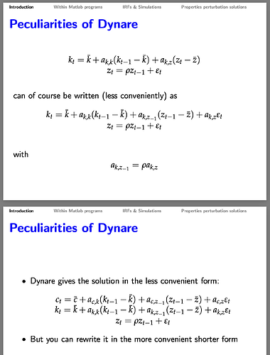
I also find this peculiarity noted in the dynare notes by Wouter J. den Haan

which is exactly what I was confused about before.

Link here: https://www.wouterdenhaan.com/numerical/slidesdynare.pdf

  1. I find it more convenient to set up the model in levels and only request output of the logged variables I really need.
  2. Starting with Dynare 6.0, if you use var(log), Dynare automatically appends the logged variable. That’s why I can access LOG_y in the simulations.
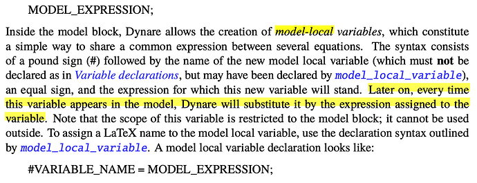
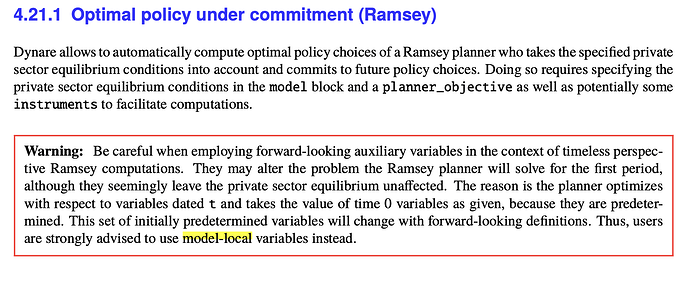
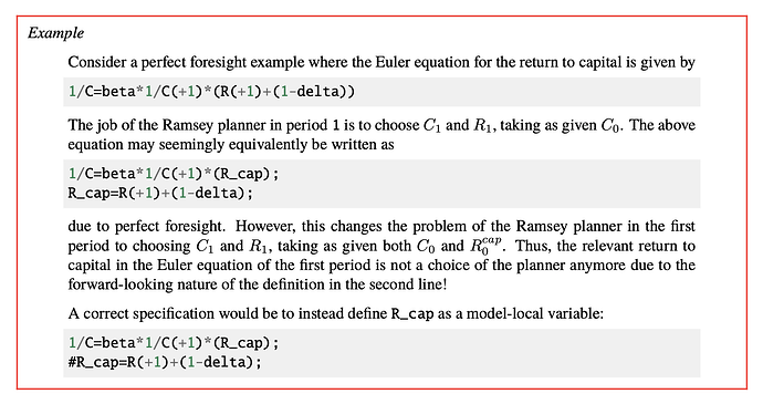
  3. The # is for model-local variables. It substitutes the expression at all occurrences in the mod-file. I use it for the SDF to prevent timing errors that create issues at higher order.
  4. You could use e.g. rng(1); to set the seed.
  5. Dynare internally only works with end of the period values. That’s what the predetermined_variables command does. The t index denotes all variables in the current information set, i.e. after seeing the realizations of today’s shocks. But yes, your description is correct.
  6. Yes, that would work.
1 Like

Yes, you are correct. The Dynare implementation is more cumbersome but also more general, e.g. at higher order.

1 Like

Thank you so much! I benefit so much from your careful responses.

For my own and others’ reference:

Just to follow up on model-local variables, I find in they Dynare 6.1 manual

Also the following example:


A tiny follow-up on this part:

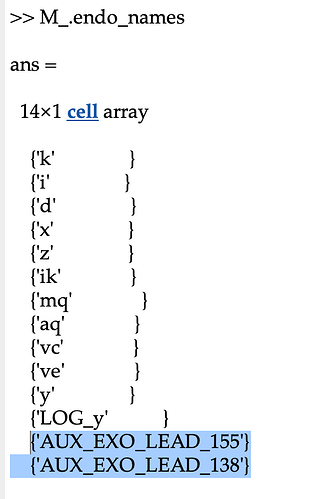
When I look at the list of variables in the model, I dont recognize the last two at all. Are they exogenous shocks?

Thanks.

Kind of. See

thank you for the reference, which is helpful

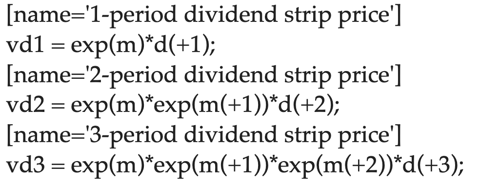
How may I compute something like the following:

P^n_t = E_t[ (M_{t+1}M_{t+2}...M_{t+n})D_{t+n} ]

I tried in this code, it only works for n=1, perhaps due to the setup of M in the code.

But it does not work due to m