Dear all,
I am totally new with Dynare and I am trying to replicate in Dynare the DSGE model of Uribe (2018) from this article: Uribe (2019), The Neo-Fisher Effect, Econometric Evidence from Empirical and Optimizing Model.pdf (326.7 KB). I reported the parameter values (p.33-34) as my starting values and I manage to complete my model block and my initval block. The problem is when I run the resid(1) command for the residuals of the static equations, one equation is not equal to zero. Maybe I have an error in my model block, but I can’t find it. I don’t know if it’s because of this but my results when i run the stoch_simul are far from Uribe (2019). Can you help me with this?
Uribe Matlab code : www.columbia.edu/~mu2166/neoFisher/index.htm
(particularly the nk_ss.m file and the nk_model.m file from optimizing.zip)
My .mod file: uribe2019_v030820.mod (2.9 KB)
Thanks
Hello everyone,
I still have the same problem, I search in this forum and in the Dynare manual but could not find an answer.
Can anyone could help me with this?
Best regards
To aid debugging, I would suggest to make use of Dynare’s \LaTeX-capabilties and tagging the equations to see what you implemented.
Hi,
First of all thank you for your answer. With the use of the Latex command and with a steady state file I managed to solve my first problem (all resid(1) = 0 now and the steady state looks good).
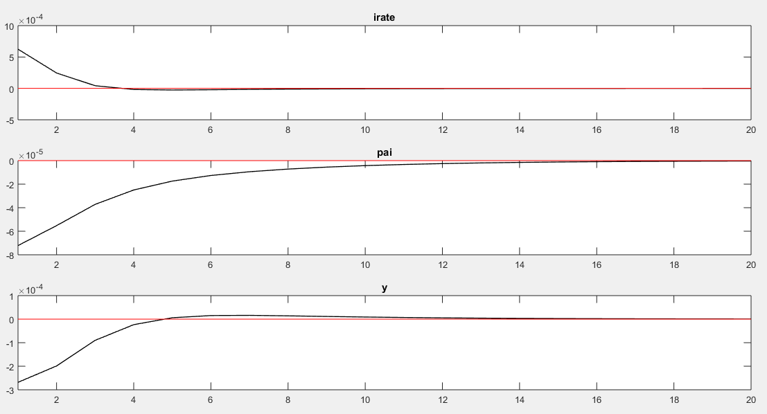
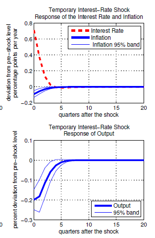
However, my results (IRFs and variance decomposition) are still differents from Uribe (p.37-38). I suspect errors in my shocks block since the direction of the IRFs is good but not the magnitude (see pictures) . I tried the relative_irf option without success. Do you have any idea what could be the problem?
new mod file: uribe_v110820.mod (3.2 KB)
steady_state file: uribe_v110820_steadystate.m (3.9 KB)
My IRFs:
Uribe:
You need to define auxiliary variables for:
- log output (to consider percent deviations)
- the annualized interest rate instead of the quarterly one
Hello professor,
thank you again for your help. I just want to clarify exactely what I need to do for each point.
-
I search in this forum for auxiliary variables to consider percent deviations and I found two way to do this. The first one is to do yhat = log(y) (as in https://github.com/JohannesPfeifer/DSGE_mod/blob/master/RBC_baseline/RBC_baseline.mod) and add yhat to my stoch simul.
The second method is to do yhat2 = log(y) -log(steady_state(y)) (as in https://github.com/JohannesPfeifer/DSGE_mod/blob/master/Jermann_Quadrini_2012/Jermann_Quadrini_2012_RBC/Jermann_Quadrini_2012_RBC.mod) and add yhat2 to my stoch simul.
Wich one I should use?
-
For the interest rate and the inflation variables, to obtain the deviation from pre-shock level in percentage points per year should I only add auxiliary variables like: iratehat = irate * 4 and inflation = inflation * 4? Or should I do something more like: iratehat2 = log(irate) -log(steady_state(irate)) * 4?
Finally I have some difficulties to implement the permanent interest shock. I need to insure that the initial shock increases the permanent component of the interest rate and inflation by 0.25 percent per quarter or 1 percent per year. Is there an easy way to do this in Dynare like the endval command in deterministic model?
Thank you again for your useful help!