Understanding the Bayesian Computation of Smets Wouters (2007)

numpynp · May 23, 2024, 6:35am

Hi everyone! My ultimate objective is to understand the Bayesian computational background behind Smets-Wouters (2007), and I have two questions related to this big objective.
A
Almost directly building on Johannes’ SW code on github, I was trying to diagnose whether the SmetsWouters 2007 Bayesian method (Random Walk MH algorithm) appropriately converged or not, and wanted to plot a autocorrelogram using

estimation(optim=('MaxIter',200),datafile='../../source/raw/orig/usmodel_data',dirname='../../output/analysis/',mode_file=usmodel_mode,mode_compute=0,first_obs=1, presample=4,lik_init=2,prefilter=0,mh_replic=20000,mh_nblocks=2,mh_jscale=0.20,mh_drop=0.2, nograph, nodiagnostic, tex);

mh_autocorrelation_function(options_,M_,estim_params_,'StructuralShock',2,'csadjcost','csigma')

, where I wanted to plot two variables “csadjcost” and “csigma” in the model. But I get an error “The correlation between csadjcost and csigma is not an estimated parameter”

B Is there a nice suite of files that implement a toy model version of the original Smets-Wouters (2007), using the same core estimation technique of Bayesian MCMC, but with significantly fewer variables and hopefully many visualizations and intuition, where I can really play around and understand what is going on.

I have attached the general code files in my directory(very messy…) in case that is useful.
SW_2007_modified_public_0522.zip

jpfeifer · May 23, 2024, 8:02am

csigma for example is not a StructuralShock but a DeepParameter. You also need to generate one plot for each parameter.
Which type of toy model did you have in mind? I tend to use DSGE_mod/RBC_baseline at master · JohannesPfeifer/DSGE_mod · GitHub for teaching.

numpynp · May 26, 2024, 1:36am

Thank you Professor for the reply!

Regarding Question A
I modified the code to only focus on one Structural Shock parameter ‘csadjcost’,
i.e.,

mh_autocorrelation_function(options_,M_,estim_params_,'StructuralShock',2,'csadjcost','csadjcost')

but I still get the “not an estimated parameter” error, as the output below shows (I also tried “mh_autocorrelation_function(options_,M_,estim_params_,‘StructuralShock’,2,‘csadjcost’)”, with no success) ).

Starting Dynare (version 5.5).
Calling Dynare with arguments: none
Starting preprocessing of the model file ...
WARNING: in the 'steady_state_model' block, variable 'ewma' is not assigned a value
WARNING: in the 'steady_state_model' block, variable 'epinfma' is not assigned a value
WARNING: in the 'steady_state_model' block, variable 'zcapf' is not assigned a value
WARNING: in the 'steady_state_model' block, variable 'rkf' is not assigned a value
WARNING: in the 'steady_state_model' block, variable 'kf' is not assigned a value
WARNING: in the 'steady_state_model' block, variable 'pkf' is not assigned a value
WARNING: in the 'steady_state_model' block, variable 'cf' is not assigned a value
WARNING: in the 'steady_state_model' block, variable 'invef' is not assigned a value
WARNING: in the 'steady_state_model' block, variable 'yf' is not assigned a value
WARNING: in the 'steady_state_model' block, variable 'labf' is not assigned a value
WARNING: in the 'steady_state_model' block, variable 'wf' is not assigned a value
WARNING: in the 'steady_state_model' block, variable 'rrf' is not assigned a value
WARNING: in the 'steady_state_model' block, variable 'mc' is not assigned a value
WARNING: in the 'steady_state_model' block, variable 'zcap' is not assigned a value
WARNING: in the 'steady_state_model' block, variable 'rk' is not assigned a value
WARNING: in the 'steady_state_model' block, variable 'k' is not assigned a value
WARNING: in the 'steady_state_model' block, variable 'pk' is not assigned a value
WARNING: in the 'steady_state_model' block, variable 'c' is not assigned a value
WARNING: in the 'steady_state_model' block, variable 'inve' is not assigned a value
WARNING: in the 'steady_state_model' block, variable 'y' is not assigned a value
WARNING: in the 'steady_state_model' block, variable 'lab' is not assigned a value
WARNING: in the 'steady_state_model' block, variable 'pinf' is not assigned a value
WARNING: in the 'steady_state_model' block, variable 'w' is not assigned a value
WARNING: in the 'steady_state_model' block, variable 'r' is not assigned a value
WARNING: in the 'steady_state_model' block, variable 'a' is not assigned a value
WARNING: in the 'steady_state_model' block, variable 'b' is not assigned a value
WARNING: in the 'steady_state_model' block, variable 'g' is not assigned a value
WARNING: in the 'steady_state_model' block, variable 'qs' is not assigned a value
WARNING: in the 'steady_state_model' block, variable 'ms' is not assigned a value
WARNING: in the 'steady_state_model' block, variable 'spinf' is not assigned a value
WARNING: in the 'steady_state_model' block, variable 'sw' is not assigned a value
WARNING: in the 'steady_state_model' block, variable 'kpf' is not assigned a value
WARNING: in the 'steady_state_model' block, variable 'kp' is not assigned a value
Found 40 equation(s).
Evaluating expressions...done
Computing static model derivatives (order 1).
Computing dynamic model derivatives (order 2).
Processing outputs ...
done
Preprocessing completed.


You did not declare endogenous variables after the estimation/calib_smoother command.

Warning: Some of the parameters have no value (ccs, cinvs, crdpi) when using initial_estimation_checks. If these parameters are not initialized in a
steadystate file or a steady_state_model-block, Dynare may not be able to solve the model. Note that simul, perfect_foresight_setup, and
perfect_foresight_solver do not automatically call the steady state file. 
Initial value of the log posterior (or likelihood): -1484.2789

RESULTS FROM POSTERIOR ESTIMATION
parameters
           prior mean     mode    s.d.  prior pstdev

crhoa          0.5000   0.9826  0.0044   beta 0.2000 
crhob          0.5000   0.1391  0.0815   beta 0.2000 
crhog          0.5000   0.9686  0.0102   beta 0.2000 
crhoqs         0.5000   0.6121  0.0549   beta 0.2000 
crhoms         0.5000   0.1999  0.0639   beta 0.2000 
crhopinf       0.5000   0.9856  0.0084   beta 0.2000 
crhow          0.5000   0.9818  0.0092   beta 0.2000 
cmap           0.5000   0.8340  0.0568   beta 0.2000 
cmaw           0.5000   0.9337  0.0203   beta 0.2000 
csadjcost      4.0000   6.3144  0.9475   norm 1.5000 
csigma         1.5000   1.2679  0.1135   norm 0.3750 
chabb          0.7000   0.8056  0.0391   beta 0.1000 
cprobw         0.5000   0.7668  0.0374   beta 0.1000 
csigl          2.0000   2.5201  0.5816   norm 0.7500 
cprobp         0.5000   0.5304  0.0462   beta 0.1000 
cindw          0.5000   0.5345  0.1060   beta 0.1500 
cindp          0.5000   0.1779  0.0784   beta 0.1500 
czcap          0.5000   0.3597  0.0991   beta 0.1500 
cfc            1.2500   1.6670  0.0728   norm 0.1250 
crpi           1.5000   1.8685  0.1640   norm 0.2500 
crr            0.7500   0.8739  0.0167   beta 0.1000 
cry            0.1250   0.1203  0.0257   norm 0.0500 
crdy           0.1250   0.1282  0.0194   norm 0.0500 
constepinf     0.6250   0.6365  0.0982   gamm 0.1000 
constebeta     0.2500   0.1126  0.0457   gamm 0.1000 
constelab      0.0000   1.3263  0.8422   norm 2.0000 
ctrend         0.4000   0.5113  0.0135   norm 0.1000 
cgy            0.5000   0.5881  0.0859   norm 0.2500 
calfa          0.3000   0.2024  0.0180   norm 0.0500 

standard deviation of shocks
           prior mean     mode    s.d.  prior pstdev

ea             0.1000   0.5017  0.0263   invg 2.0000 
eb             0.1000   0.3583  0.0305   invg 2.0000 
eg             0.1000   0.6752  0.0323   invg 2.0000 
eqs            0.1000   0.5678  0.0554   invg 2.0000 
em             0.1000   0.2290  0.0121   invg 2.0000 
epinf          0.1000   0.2181  0.0235   invg 2.0000 
ew             0.1000   0.2663  0.0180   invg 2.0000 


Log data density [Laplace approximation] is -1571.472030.

Estimation::mcmc: Multiple chains mode.
Estimation::mcmc: Old mh-files successfully erased!
Estimation::mcmc: Old metropolis.log file successfully erased!
Estimation::mcmc: Creation of a new metropolis.log file.
Estimation::mcmc: Searching for initial values...
Estimation::mcmc: Initial values found!

Estimation::mcmc: Write details about the MCMC... Ok!
Estimation::mcmc: Details about the MCMC are available in ../../output/analysis//metropolis\Smets_Wouters_2007_45_mh_history_0.mat


Estimation::mcmc: Number of mh files: 1 per block.
Estimation::mcmc: Total number of generated files: 2.
Estimation::mcmc: Total number of iterations: 20000.
Estimation::mcmc: Current acceptance ratio per chain: 
                                                       Chain  1: 50.84%
                                                       Chain  2: 51.28%
Estimation::mcmc: Total number of MH draws per chain: 20000.
Estimation::mcmc: Total number of generated MH files: 1.
Estimation::mcmc: I'll use mh-files 1 to 1.
Estimation::mcmc: In MH-file number 1 I'll start at line 4001.
Estimation::mcmc: Finally I keep 16000 draws per chain.

Estimation::marginal density: I'm computing the posterior mean and covariance...  Done!
Estimation::marginal density: I'm computing the posterior log marginal density (modified harmonic mean)... Done!


ESTIMATION RESULTS

Log data density is -1573.214668.

parameters
             prior mean   post. mean        90% HPD interval    prior       pstdev

crhoa             0.500       0.9807      0.9734      0.9881     beta       0.2000
crhob             0.500       0.2156      0.0420      0.3854     beta       0.2000
crhog             0.500       0.9666      0.9504      0.9827     beta       0.2000
crhoqs            0.500       0.6313      0.5432      0.7266     beta       0.2000
crhoms            0.500       0.2053      0.1004      0.3005     beta       0.2000
crhopinf          0.500       0.9790      0.9638      0.9950     beta       0.2000
crhow             0.500       0.9779      0.9637      0.9925     beta       0.2000
cmap              0.500       0.8288      0.7454      0.9134     beta       0.2000
cmaw              0.500       0.9235      0.8902      0.9575     beta       0.2000
csadjcost         4.000       6.3649      4.6691      8.1499     norm       1.5000
csigma            1.500       1.2550      1.0745      1.4581     norm       0.3750
chabb             0.700       0.7878      0.7129      0.8648     beta       0.1000
cprobw            0.500       0.7649      0.7070      0.8236     beta       0.1000
csigl             2.000       2.5218      1.5494      3.4186     norm       0.7500
cprobp            0.500       0.5555      0.5001      0.6067     beta       0.1000
cindw             0.500       0.5217      0.3513      0.6756     beta       0.1500
cindp             0.500       0.2053      0.0749      0.3283     beta       0.1500
czcap             0.500       0.3788      0.2430      0.5352     beta       0.1500
cfc               1.250       1.6601      1.5321      1.7697     norm       0.1250
crpi              1.500       1.8984      1.6339      2.1606     norm       0.2500
crr               0.750       0.8759      0.8507      0.9019     beta       0.1000
cry               0.125       0.1263      0.0816      0.1651     norm       0.0500
crdy              0.125       0.1365      0.1013      0.1728     norm       0.0500
constepinf        0.625       0.6558      0.5017      0.8087     gamm       0.1000
constebeta        0.250       0.1365      0.0509      0.2227     gamm       0.1000
constelab         0.000       1.1582     -0.1792      2.4801     norm       2.0000
ctrend            0.400       0.5060      0.4817      0.5279     norm       0.1000
cgy               0.500       0.5971      0.4493      0.7470     norm       0.2500
calfa             0.300       0.2018      0.1717      0.2309     norm       0.0500

standard deviation of shocks
             prior mean   post. mean        90% HPD interval    prior       pstdev

ea                0.100       0.5054      0.4645      0.5486     invg       2.0000
eb                0.100       0.3431      0.2794      0.4136     invg       2.0000
eg                0.100       0.6794      0.6289      0.7298     invg       2.0000
eqs               0.100       0.5536      0.4643      0.6435     invg       2.0000
em                0.100       0.2317      0.2131      0.2519     invg       2.0000
epinf             0.100       0.2171      0.1786      0.2518     invg       2.0000
ew                0.100       0.2639      0.2347      0.2936     invg       2.0000
The correlation between csadjcost and csadjcost is not an estimated parameter!

Estimation::mcmc: Total number of MH draws per chain: 20000.
Estimation::mcmc: Total number of generated MH files: 1.
Estimation::mcmc: I'll use mh-files 1 to 1.
Estimation::mcmc: In MH-file number 1 I'll start at line 4001.
Estimation::mcmc: Finally I keep 16000 draws per chain.

Regarding Question B:
Thank you very much, I took a look at those informative files. I think I am looking for some material to understand (in the relative and absolute sense) the ill-posedness of Bayesian-DSGE’s and Smets-Wouters(SW) in particular.
For example, I noticed the following features when I was running SW:
(a) the acceptance ratio is pretty high 0.5-0.6 (ideal number is usually around 0.25?)
(b) I sampled many draws of the parameters (about 45 of them) from the posterior, and saw many of the parameter draws(about 15 out of 45) were basically degenerate or NAN (e.g., curvw and curvp being always 10, ccs, cinvs, crdpi being NAN, etc.)
Relatedly, the matrix of posterior_draws is naturally nonsingular, even after excluding completely degenerate parameters.
(c) Trying to fit a normal approximation to the (log) likelihood using moment matching, the error was still nonneglible

I’m still new in this field, and I was trying to learn by reading, e.g., An and Schorfheide 2007, but I haven’t seen much specifically targeted towards SW.

Any specific/general remarks on these issues would be much appreciated!

jpfeifer · May 27, 2024, 11:58am

As a I wrote above, it should be

mh_autocorrelation_function(options_,M_,estim_params_,'DeepParameter',2,'csadjcost','csadjcost')

The acceptance rate should be about 0.25 but other numbers are also acceptable. You may need more draws in that case.
Draws from the posterior should never be degenerate. These draws should be discarded on a priori grounds.

numpynp · May 28, 2024, 2:41am

Thank you professor for the response!
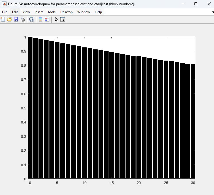
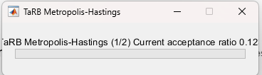
Re 1(and 2) The autocorrelogram code works now, but the problem is that most parameters have over 0.8-0.9 autocorrelation, way too high, aligning with the problematic acceptance rate (>0.5).
As you suggested in 2., I thought maybe the number of samples were insufficient, so I increased the number of simulations per block from 20,000 to 60,000( i have 2 blocks), but there was barely no change in the acceptance ratio and autocorrelogram… Do you think it is ok to conclude from this that SW 2007 is ill-posed for Bayesian computation? Are there any other approaches I might take?

Re 3[First point].
Thank you, I am wondering then if the degeneracy might have something to do with the way I’m setting up the parameters in dynare?
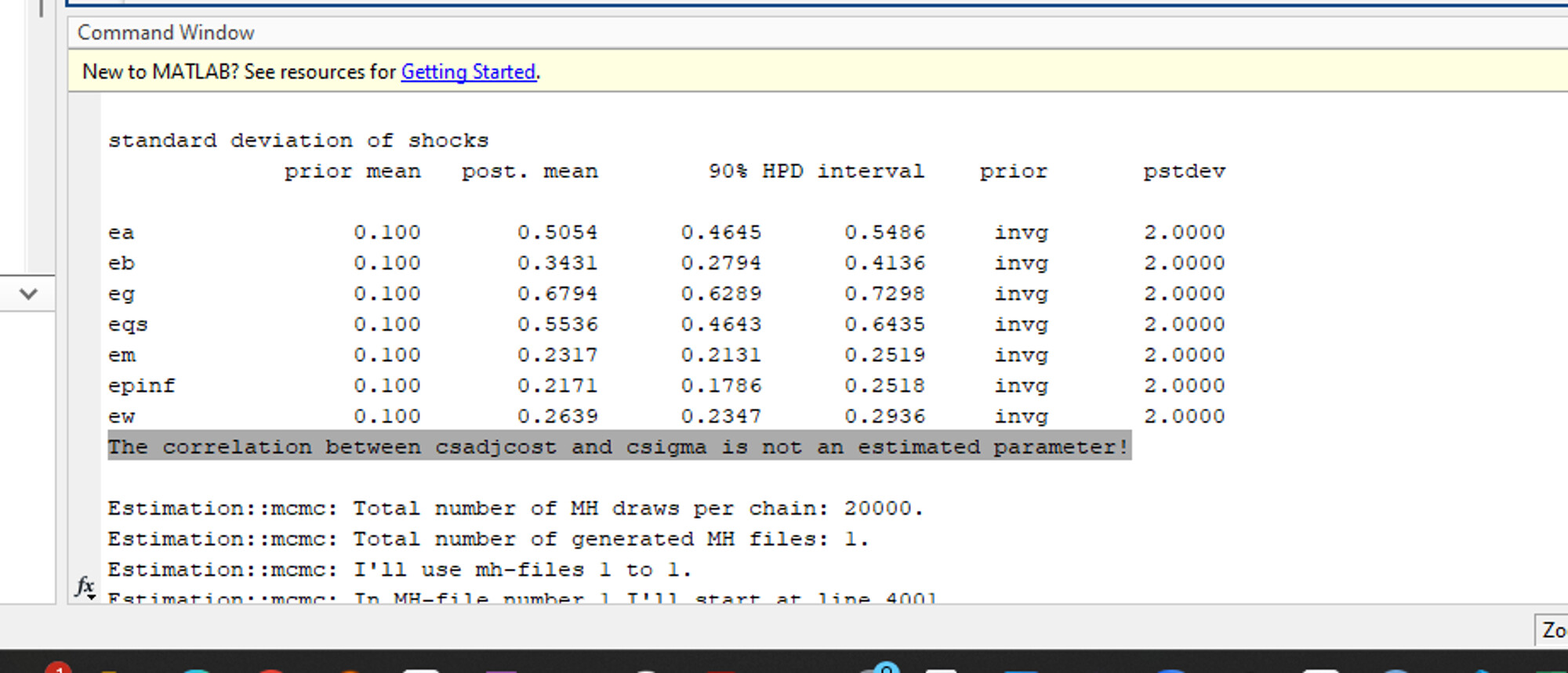
For example, I get the below warning every time I run the code that your group has provided for SW 2007:

Starting Dynare (version 5.5).
Calling Dynare with arguments: none
Starting preprocessing of the model file ...
WARNING: in the 'steady_state_model' block, variable 'ewma' is not assigned a value
WARNING: in the 'steady_state_model' block, variable 'epinfma' is not assigned a value
WARNING: in the 'steady_state_model' block, variable 'zcapf' is not assigned a value
WARNING: in the 'steady_state_model' block, variable 'rkf' is not assigned a value
WARNING: in the 'steady_state_model' block, variable 'kf' is not assigned a value
WARNING: in the 'steady_state_model' block, variable 'pkf' is not assigned a value
WARNING: in the 'steady_state_model' block, variable 'cf' is not assigned a value
WARNING: in the 'steady_state_model' block, variable 'invef' is not assigned a value
WARNING: in the 'steady_state_model' block, variable 'yf' is not assigned a value
WARNING: in the 'steady_state_model' block, variable 'labf' is not assigned a value
WARNING: in the 'steady_state_model' block, variable 'wf' is not assigned a value
WARNING: in the 'steady_state_model' block, variable 'rrf' is not assigned a value
WARNING: in the 'steady_state_model' block, variable 'mc' is not assigned a value
WARNING: in the 'steady_state_model' block, variable 'zcap' is not assigned a value
WARNING: in the 'steady_state_model' block, variable 'rk' is not assigned a value
WARNING: in the 'steady_state_model' block, variable 'k' is not assigned a value
WARNING: in the 'steady_state_model' block, variable 'pk' is not assigned a value
WARNING: in the 'steady_state_model' block, variable 'c' is not assigned a value
WARNING: in the 'steady_state_model' block, variable 'inve' is not assigned a value
WARNING: in the 'steady_state_model' block, variable 'y' is not assigned a value
WARNING: in the 'steady_state_model' block, variable 'lab' is not assigned a value
WARNING: in the 'steady_state_model' block, variable 'pinf' is not assigned a value
WARNING: in the 'steady_state_model' block, variable 'w' is not assigned a value
WARNING: in the 'steady_state_model' block, variable 'r' is not assigned a value
WARNING: in the 'steady_state_model' block, variable 'a' is not assigned a value
WARNING: in the 'steady_state_model' block, variable 'b' is not assigned a value
WARNING: in the 'steady_state_model' block, variable 'g' is not assigned a value
WARNING: in the 'steady_state_model' block, variable 'qs' is not assigned a value
WARNING: in the 'steady_state_model' block, variable 'ms' is not assigned a value
WARNING: in the 'steady_state_model' block, variable 'spinf' is not assigned a value
WARNING: in the 'steady_state_model' block, variable 'sw' is not assigned a value
WARNING: in the 'steady_state_model' block, variable 'kpf' is not assigned a value
WARNING: in the 'steady_state_model' block, variable 'kp' is not assigned a value
Found 40 equation(s).
Evaluating expressions...done
Computing static model derivatives (order 1).
Computing dynamic model derivatives (order 2).
Processing outputs ...
done
Preprocessing completed.


You did not declare endogenous variables after the estimation/calib_smoother command.

[Warning: Some of the parameters have no value (ccs, cinvs, crdpi) when using initial_estimation_checks. If these
parameters are not initialized in a steadystate file or a steady_state_model-block, Dynare may not be able to solve the
model. Note that simul, perfect_foresight_setup, and perfect_foresight_solver do not automatically call the steady state
file.] 
Initial value of the log posterior (or likelihood): -1484.2789

Re 3[2nd point].Relatedly, to dive into this issue in a more tractable way, I am starting with your suggested RBC_baseline material DSGE_mod/RBC_baseline at master · JohannesPfeifer/DSGE_mod · GitHub
and trying to get multiple draws from the posterior as well as the likelihood evaluated at that parameter value by using the dsge_likelihood function, but the problem I have now is I dont have a way to see the “info” variable from the dsge_likelihood (which is important because that output shows whether the kalman filter’s matrices are nonsingular or not).
Specifically,
as if I use the

posterior_function(function=‘OOI_and_likelihood’,sampling_draws=100) as a wrapper, I can’t seem to be able to recover the “info” output,
and on the other hand, if I
add the code in the attached file “RBC_baseline_first_diff_bayesian.mod”(I added some lines to your original code),

[fval, info] = dsge_likelihood(xparam1,dataset_,dataset_info,options_,M_,estim_params_,bayestopt_,prior_bounds(bayestopt_, options_.prior_trunc),oo_)

returns the error

Unrecognized function or variable 'xparam1'.

Error in RBC_baseline_first_diff_bayesian.driver (line 329)
[fval, info] = dsge_likelihood(xparam1,dataset_,dataset_info,options_,M_,estim_params_,bayestopt_,prior_bounds(bayestopt_, options_.prior_trunc),oo_)

Error in dynare (line 281)
    evalin('base',[fname '.driver']);

Error in yp_script_basic (line 3)
dynare RBC_baseline_first_diff_bayesian.mod

although in examples I saw online, the xparam1 was being used.

Thank you so much for your time!

jpfeifer · May 28, 2024, 4:55pm

High autocorrelation is not an issue per se. It just means each single draw will contain less new information than an iid draw. That’s why you can simply use more draws (and potentially do some thinning).
I would not call this degeneracy. The posterior sampling algorithms belong to the class of Monte Carlo Markov Chain algorithms. As the name “Markov Chain” suggests, there is always some dependency. That being said, you can often tweak the MCMC sampler to show less autocorrelation, e.g. by improving the scaling matrix or using a different sampler than the Random Walk Metropolis-Hastings.
The following function works in Dynare 6.1:
OOI_and_likelihood.m (3.6 KB)

numpynp · June 1, 2024, 2:33am

Thank you professor!
Re. 1 and 2, I have been spending a few days trying to tune the parameters in the estimation() to make the SW 2007 be better behaved, but not succeeding well. Do you have prior knowledge on the exact method/values I should choose specifically for SW 2007? I couldn’t find anything specific in the literature, which I’m a bit surprised of given it being so commonly used…

jpfeifer · June 3, 2024, 9:25am

The model can be tricky to work with. See e.g.
https://www.sciencedirect.com/science/article/pii/S0304407609001900

numpynp · June 6, 2024, 2:23am

Thank you Professor for the suggestion, I am reading/processing the paper now!

Simultaneously, based on your previous suggestion to use your RBC baseline model to understand fundamentals of DSGE Bayesian computation, I have used that to get the posterior draws from it using the posterior_function() that ultimately uses the dsge_likelihood() under the hood. I currently have the following concern/problems.
(a)
I saved the posterior_draws result in the excel sheet(as in the attached file), but I get the below values, where except rhoz and rhog, they are all constant. Is the variable “log_likelihood” correctly dealing with those constant variables?

(b)
For SW 2007 posterior_draws log_likelihood, it was all around -1400, whereas for the RBC_baseline case, it has the opposite sign of about 1400 for each observation. This is not a coding error but theoretically legitimate, I hope?

My folder including code based on RBC_Baseline is available here

jpfeifer · June 6, 2024, 7:57am

For the RBC model, we have

estimated_params;
rhog, beta_pdf,0.7,0.1;
rhoz, beta_pdf,0.7,0.1;
stderr eps_z, inv_gamma_pdf, 0.01, 0.1;
stderr eps_g, inv_gamma_pdf, 0.01, 0.1;
end;

Those are the only estimated parameters. Everything else is fixed.
2. The sign can be positive or negative. See

numpynp · June 7, 2024, 2:17pm

Thank you professor!

Re. 1, I’m still confused in two respects:
(a)
Comparing the remarks

and

I’m not sure if you are saying my current excel file, and the log_likelihood value(the second to last column) is valid or not. I basically directly inserted the results from the default “oo_.posterior_function_results”, which was obtained by

[fval, info] = dsge_likelihood(xparam1,dataset_,dataset_info,options_,M_,estim_params_,bayestopt_,bounds,oo_);

Should I have somehow apriori discarded those constant variables before having them appear in the “oo_.posterior_function_results”?

(b) Also concerningly, as in my screenshot of the excel sheet above, the posterior_draws do not include the “stderr eps_z”, “stderr eps_g”. Is this a bug in my code, or the default behavior of Dynare? How do I interpret the column “log_likelihood” then? Is it still the joint log likelihood of “rhoz”, “rhog”, “stderr eps_z”, “stderr eps_g” or just the marginal log likelihood of “rhoz” and “rhog”, or something else?

Two more questions in relation to some of our previous iterations

I’m trying the suggested tailored randomized block algorithm in the SW model for 4 hours, but the progress bar has not changed at all. I know it takes much more time, but is something going wrong?

When I want to conduct a normal approximation to the posterior density (i.e., find the mean and var-cov matrix parametter) with the objective of minimizing the KL divergence, what method would be the best? I think the laplace approximation is the most common method, but that just simply matches the mode and uses the second-order taylor approximation, and there is no guarantee that minimizes the KL?

jpfeifer · June 10, 2024, 5:43pm

I was saying that degeneracy is not the problem here. You are estimating exactly two structural parameters, keeping all other parameters fixed. For that reason, only those two parameters vary with the MCMC draws.
The standard deviations parameters are still estimated but stored in M_.Sigma_e. Thus, it’s the joint likelihood.
How many draws did you set for the TaRB?
I am not sure I understand the question. The normal distribution is completely characterized by the first two moments. Those are the ones you want to match.

numpynp · June 16, 2024, 10:43am

Thank you Professor, it seems there were a couple of misunderstandings on my end, and your comments clarified many of them. I am still working on the TaRB, but will let you know if I come up with more specific questions, thanks again!