Hi!
I have built a model for a small open economy within a currency union. The model runs in dynare, however, a historical shock decomposition produces strange graphs. The same is true for the IRFs.
These problems might be related to the assumptions made for this small open economy. I have assumed that there is a common monetary policy, that imports enter the goods market equilibrium of the small economy, but not of the large economy and that imported inflation only plays a role in the small economy, but not for the large economy. Monetary policy, however, responds to overall inflation and output gap, weighted with the respective country shares.
Since it is a currency union, there is only a real exchange rate, but no nominal exchange rate in the model. The real exchange rate is defined as the difference in inflation rates. I have also tried to determine the real exchange rate via the uncovered interest parity, but this does not change the results (strange graphs). My way to model the open economy for two countries works for the canonical 3-equation-version, but it does not work, once I have moved to a more complex framework.
I hope you can give me hints how to appropriately link the two countries.
Please find attached the mod-file
model3b.mod (3.1 KB)
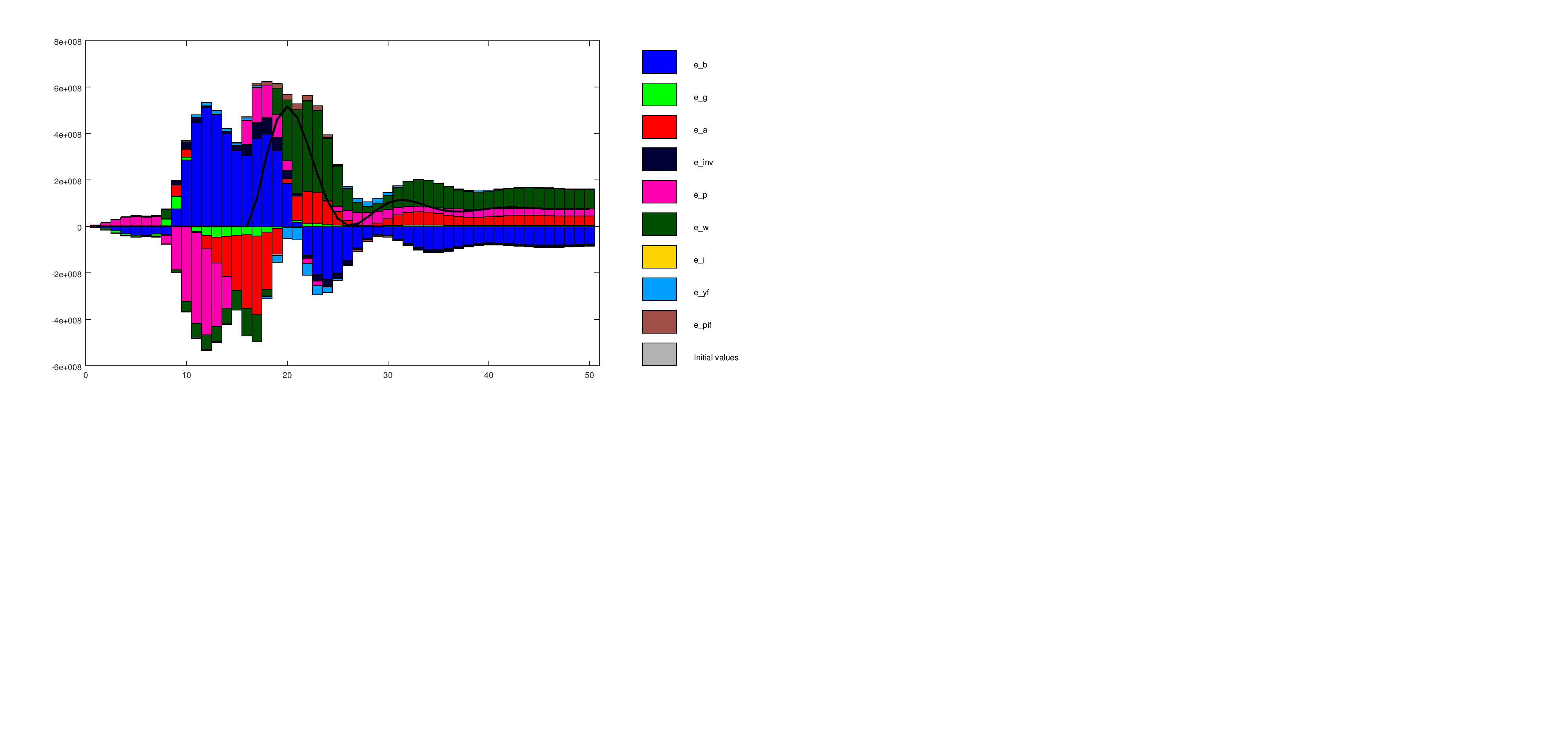
The strange thing is that I get these shock decomposition graphs. It’s not entirely clear, whether this stems from computational errors or from the model assumptions.
The standard open economy framework for New Keynesian DSGE models seems to be Gali/Monacelli and this works perfectly in the context of the 3-equation model. However, when I move to a Smets/Wouters-style model with investment and labor under the assumption of a fixed exchange rate, it no longer works. Why is that the case?
Your model is wrong. Using model_diagnostics returrns
MODEL_DIAGNOSTICS: The following endogenous variables aren’t present at the current period in the model:
k
On top of that, your model seems to have an improperly handled constant term in equation 19. Due to linearization, your model variables should all have a steady state of 0. But your Taylor rule contains a constant term pi_target that should not be there in this form. This causes the weird steady state.
Thank you for your reply… But after correction of the two mistakes, I get the following error message:
Blockquote
ꔽEIGENVALUES:
Modulus Real Imaginary
      0.1329           0.1329                0
      0.2837           0.2837                0
         0.5              0.5                0
         0.5              0.5                0
         0.5              0.5                0
         0.5              0.5                0
         0.5              0.5                0
         0.5              0.5                0
         0.5              0.5                0
         0.5              0.5                0
         0.5              0.5                0
      0.6672           0.6653          0.04953
      0.6672           0.6653         -0.04953
      0.8386           0.7033           0.4568
      0.8386           0.7033          -0.4568
      0.9985           0.9985                0
       1.039            1.039                0
       1.493            1.452           0.3488
       1.493            1.452          -0.3488
       1.808            1.732           0.5188
       1.808            1.732          -0.5188
       3.585            3.585                0
  1.586e+016      -1.586e+016                0
  7.642e+016      -7.642e+016                0
There are 8 eigenvalue(s) larger than 1 in modulus
for 9 forward-looking variable(s)
The rank condition ISN’T verified!
Blanchard Kahn conditions are not satisfied: indeterminacy
How can I correct this?
You need to figure out the correct timing in your model. I guess you changed the timing of k for it to appear contemporaneously. But there must still be something wrong as the Blanchard-Kahn conditions are not satisfied.
The BK conditions are no longer satisfied, if k is not predetermined. Once k is predetermined, the BK conditions are satisfied, but then the model produces weird graphs. I guess there is somewhere a coding mistake, because from the point of economic intuition/theory my model makes sense.
I don’t understand your issue. Of course, k is a predetermined variable. But nevertheless it must be showing up contemporaneously.
But when I declare k as predetermined variable, I get the following message from model_diagnostics:
Blockquote
MODEL_DIAGNOSTICS: The following endogenous variables aren’t present at the current period in the model: k
The law of motion for capital, as I have defined it, is k=k1*k(-1)+(1-k1)invest+k2einv. Or should this be shifted one period forward?
You need the predetermined_variables command to shift a model entered in the stock at the beginning of period convention to Dynare’s end of the period convention. But your law of motion above is already in the end the of period notation.
So, if I have it already in the end of period notation, I do not have to declare it as predetermined, right? But in this case the BK conidtions are no longer satisfied (indeterminacy)!
Nevertheless, the model works fine in the closed economy, no matter whether k is predetermined or not.
I just would like to have a Smets/Wouters-style model, which works in the open economy context.
Then there must be something fundamentally wrong somewhere. Timing must matter, even in the closed economy version. You are correct that if you use the end of period notation, you do not have to declare the state as predetermined. That omitting this statement results in indeterminacy confirms that there is still a timing problem somewhere.
Now, one problem for the steady state results (which are never zero, except for the shocks) could be simultaneous calculation of wage and labor, which are both endogenous in my model. When I set labor to a constant parameter, the model no longer works. On the other hand, when I write output gap as the difference between the goods market equilibrium and the production function, the model says there is one equation less than endogenous variables. This implies that labour is endogenously determined by the production function, which also contains labor. Therefore, I tried to define the output gap as the difference between a sticky price and a flexible price economy, so that the number of equations matches the number of endogenous variables.
However, this gives the following error message (although this time the steady state results are now zero for all variables!):
Blockquote
EIGENVALUES:
Modulus Real Imaginary
      0.2974           0.2974                0
      0.4615           0.4615                0
         0.5              0.5                0
         0.5              0.5                0
         0.5              0.5                0
         0.5              0.5                0
         0.5              0.5                0
         0.5              0.5                0
         0.5              0.5                0
      0.6011           0.6011                0
      0.6044           0.3587           0.4865
      0.6044           0.3587          -0.4865
      0.6891           0.6891                0
      0.7549           0.7549                0
      0.9483           0.9477          0.03529
      0.9483           0.9477         -0.03529
      0.9835           0.9835                0
       1.059            1.059                0
       1.189           0.9677            0.691
       1.189           0.9677           -0.691
       1.263            1.233           0.2766
       1.263            1.233          -0.2766
       2.996            2.421            1.765
       2.996            2.421           -1.765
  1.213e+016       1.213e+016                0
         Inf             -Inf                0
         Inf             -Inf                0
         Inf             -Inf                0
There are 11 eigenvalue(s) larger than 1 in modulus
for 12 forward-looking variable(s)
The rank condition ISN’T verified!
MODEL_DIAGNOSTICS: No obvious problems with this mod-file were detected.
error: Blanchard Kahn conditions are not satisfied: indeterminacy
Once again, I have not defined k as predetermined, because it’s already in the end-of-period formulation. If it is predetermined, it makes indeed a difference, but the graphs are weird and it does not make a sense from an economic point of view. Please find attached the new model:
model2.mod (2.8 KB)
@jpfeifer
I have now found a way to model a small open economy in a currency union. However, I get the following error message:
Blockquote
There are 8 eigenvalue(s) larger than 1 in modulus
for 9 forward-looking variable(s)
The rank condition ISN’T verified!
MODEL_DIAGNOSTICS: The Jacobian of the static model is singular
MODEL_DIAGNOSTICS: there is 1 colinear relationships between the variables and the equations
Colinear variables:
c
invest
ks
k
l
yh
qq
Colinear equations
1 14 17 18 25
MODEL_DIAGNOSTICS: The singularity seems to be (partly) caused by the presence of a unit root
MODEL_DIAGNOSTICS: as the absolute value of one eigenvalue is in the range of ±1e-6 to 1.
MODEL_DIAGNOSTICS: If the model is actually supposed to feature unit root behavior, such a warning is expected,
MODEL_DIAGNOSTICS: but you should nevertheless check whether there is an additional singularity problem.
MODEL_DIAGNOSTICS: The presence of a singularity problem typically indicates that there is one
MODEL_DIAGNOSTICS: redundant equation entered in the model block, while another non-redundant equation
MODEL_DIAGNOSTICS: is missing. The problem often derives from Walras Law.
error: Blanchard Kahn conditions are not satisfied: indeterminacy
What do I have to do now?
model3.mod (2.9 KB)
The collinearity comes from the unit root. Don’t bother with it for now. You still need to correct the timing. Are you for example sure that
r=-(k-l)+w;
has the correct timing of k?
I am sure that the timing of k in r is correct. It’s the same timing that can be found in your Smets/Wouters code on your github site. The timing in the capital accumulation equation (which does not require to declare k as predetermined) and the timing of k in the effective capital stock (with variable capital utilization) also corresponds to the original SW paper as well as to your code.
If k is capital services, then the timing is correct. But I thought that ks in
ks=k(-1)+u;
is capital services.
k is capital and ks is capital services. But why should the timing change when I move from a closed economy to an open economy?
I don’t know your model, but the interest rate usually depends on capital services, not capital if there is variable utilization. That would be a problem in both closed and open economies. Please try to simplify your model to find out where the problem comes from. A first step is to eliminate variable capital utilization.
Thanks for your answer. Without variable capital utilization, the model does not work. But with variable capital utilization that influences the rental rate, I get reasonable irfs, but no shock decomposition.
Instead, there is one error message:
Blockquote
error: lyapunov_solver: operator *: nonconformant arguments (op1 is 0x0, op2 is 10x10)