Red dots in the estimation of basic NKSOE model

[magonfru1]

Hi,

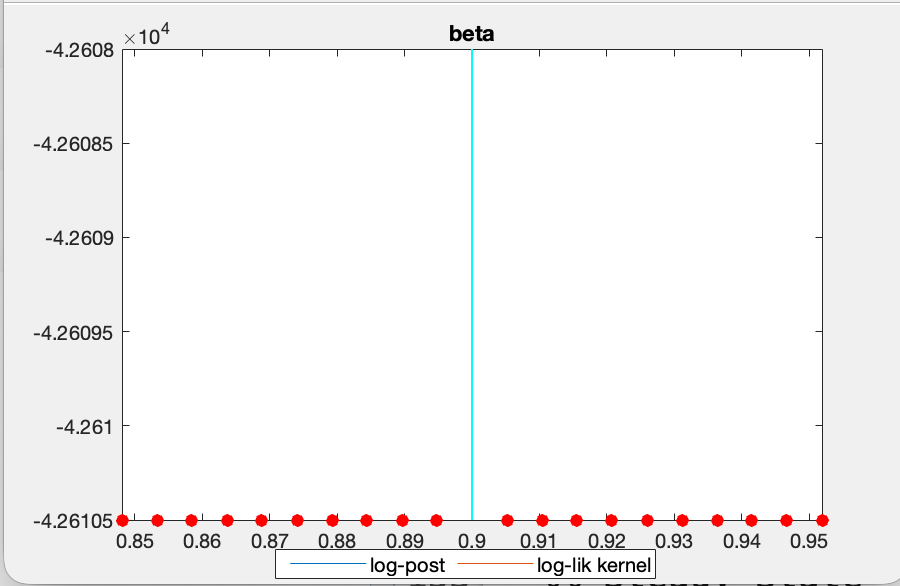
I am teaching a basic DSGE modeling class that aims that students are able to build and modify basic dsge models. In the last section of the course I am teaching a very hands on section on estimation. I got a basic NKSOE from the website of Valerio Nispi Landi, which I modify to have calvo pricing. I am trying to estimate the model using data that the Central Bank of Chile uses to estimate its large size DSGE model, however, I have found it very difficult to even find the mode. I started really small, only trying to estimate one parameter (beta) and adding (or alternating) observed series one by one, but I get red dots all around. I have read that it might be due to hitting the bounds of the parameter, but it does not seem the reason in this case. I checked model_diagnostic and the calibrated model does not seem to have any problem.

I used “beta, 0.9, , ,beta_pdf, 0.9, 0.01;” for this parameter. Something similar occurs with delta.

Then I tried to estimated the standard deviation of the shocks, but it is also giving problems. The following graph presents the productivity shock of a Cobb Douglas production function. Although in this case it finds the mode, it also shows some red dots that I don’t know how to interpret.

I have uploaded the files used in the estimation. The file contains a lot commented lines because of all the iterations.

data_XMAS_17Q2.xlsx (298.8 KB)

nk_open2.mod (9.7 KB)

[jpfeifer]

That mod-file does not handle parameter dependence correctly and cannot be used for estimation.

[magonfru1]

HI thanks, for your prompt response. Can you elaborate, please? For what I am reading, I shall use a steady state file?

Best regards

Mario

[jpfeifer]

The part

%% Steady State
piH_ss=1;
pi_ss =1;                        % inflation targeting (quarterly calibration)
d_ss  =4*D;                       % foreign debt
yH_ss =2;                        % domestic output
pH_ss =1;                        % domestic price
s_ss  =1;                         % real FX rate
h_ss  =1/3;                       % hours of work
q_ss  =1;                         % marginal value of investment (in terms of lambda)  
r_ss  =pi_ss/beta;
rk_ss =1/beta-(1-delta);         % rental rate of capital
mc_ss =(epsilon-1)/epsilon;      % real marginal costs
H_ss  = mc_ss*yH_ss*pH_ss^theta/(1-beta*omega);
F_ss  = yH_ss*pH_ss^(theta-1)/(1-beta*omega);
k_ss  = alpha*mc_ss*yH_ss/rk_ss;            % capital
w_ss  = (1-alpha)*mc_ss*yH_ss/h_ss;         % real wage
i_ss  =delta*k_ss;                   % investment
c_ss  =pH_ss*yH_ss-i_ss-pH_ss*g_ss-d_ss*(1/beta-1);       % consumption
chi   =w_ss*c_ss^-sigma/(h_ss^(phi));                      % labor preference parameter
a_ss  =yH_ss/(k_ss^(alpha)*h_ss^(1-alpha));               % tfp
gammaz=yH_ss-(1-gamma)*pH_ss^(-eta)*(c_ss+i_ss)-g_ss;   % foreign parameter
m_ss=1;

does belong in the steady_state_model block.

[magonfru1]

Awesome!

thanks, it worked