- Finding the correct mode (and all that goes into it) is the main technical challenge in estimating DSGE models. There are many intricacies. That is not a problem that is “too specific”. If you look through the forum, the non-positive definite Hessian at the mode is the most common problem in estimation. That is why I warned you long ago to embark on this path. Also keep in mind the Pareto rule: the last 20 percent take 80 percent of the time.
- Forget about the code part I wrote. Run one single estimation command with the
mode_checkoption and the graphs should show up (unless you havenographenabled). Also see Mode Check Plots Curvature - #2 by jpfeifer
But I have mode_check option included in the estimation command and still no graphs appear. I deleted your code.
Model14.mod (3.8 KB)
You commented out the estimation command.
OK, now it works. But I don’t have very clear picture in my head what does parameter hitting the bound mean. Is the bound the light blue line and parameter hitting it means that the dark red curve crosses it?
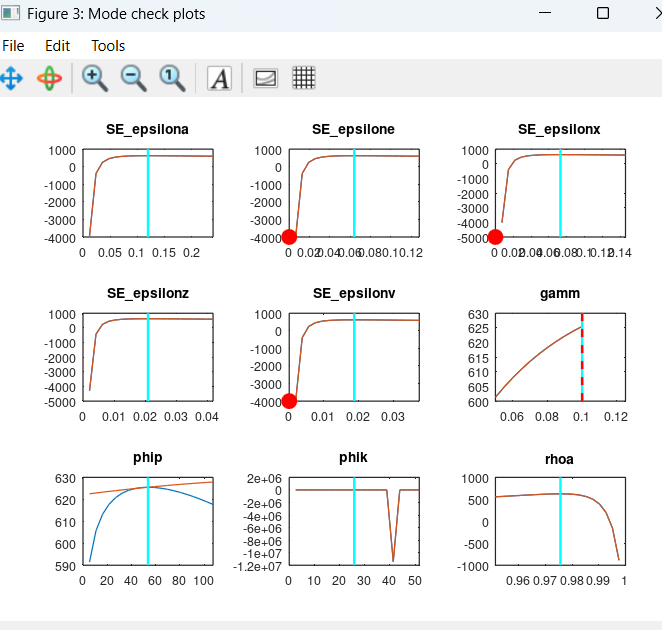
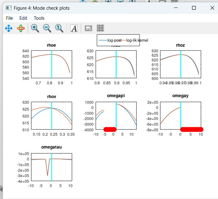
The mode (the cyan vertical line) should be at the highest point of the curves, with curves visible to both sides. If there are red dots directly to the left or right (omegapi and omegay) or nothing (gamm) you have a corner solution.
Perfect, now everything is clear. Your help is much appreciated!
So, what to do about the corner solutions?
First, I obtained an advice to use bounded parameter space. I found only one topic on this forum that mentions it without any actual code, so do you maybe have an example of it? The topic that I found:
Second, I obtained an advice to set prior_trunc=0. But it is already set in the estimation command.
As I wrote before, that is the hard part. Finding out what goes wrong. In your case, it seems the problem is both about explicit prior boundaries (gamm) and implicit prior truncation due to Blanchard-Kahn violations (the omegas). You need to better understand what is going on here. Sometimes, the data treatment/observation equations are an issue, sometimes it is just the data really being close to the indeterminacy region.
I did a bit of research.
Regarding parameters that are close to indeterminancy region, how to tell if there are economic mechanisms at work or is there a problem with data treatment? I believe an indication that the latter is the case is if the autocorrelation is high?
I’ve found an advice to revise prior means of parameters that are close to boundary.
Other people advice that the optimizer doesn’t go to the indeterminacy region if I consider a Taylor rule where the interest rate smoothing parameter affects multiplies both the previous period interest rate and inflation, output, output growth and change in the nominal exchange rate.
Yet other people advice, that during the searching of the posterior mode and Metropolis-Hastings MCMC, one needs to check whether a candidate draw is valid in every iteration. Moreover, one would like to discard any draw from indeterminancy regions during the estimation.
Second, regarding data treatment, I believe the most often forgotten are constants in the observation equation. Could you please tell me where are observation equations in the Dynare file, I believe they follow the “model;” command? Are there any variables where the mean does not match and is for any variables the variance very large?
Model10.mod (4.5 KB)
- You did not provide the corresponding data file.
- Unit roots induced by wrong observation equation (which are in the
model-block) are more about stability than indeterminacy. - Dynare of course rejects invalid parameter draws that do not satisfy the BK conditions. This is why your mode is at the boundary. It cannot go into the indeterminacy region.
- Yes, changing priors can help, but it means overriding what the data tell you. Modifying the model may be more sensible.
Here are the data files for one of the three countries estimated.
Slovenia.xlsx (15.9 KB)
Slovenia.mat (10.9 KB)
Slovenia.m (10.9 KB)
Dear professor,
have you maybe had a chance to look at my data files, that you asked for? I was wondering, is there a problem with data treatment? Thank you in advance!
From what I can see, the data treatment looks correct.
Perfect, thank you so much.
So, this means there is a problem either with observation equations in the model block or with data close to interdeterminancy region. How to tell which is the case?
Perhaps, I should check if autocorrelation is high? Or are there any forgotten constants in the observation equations?
Have you tried working with demeaned observations and mapping them to deviations from steady state in the model?
Not yet, thanks for the idea.
But you said that data (treatment) looks correct. So should I demean (deduct mean from) every value in my real world observations file (panel data including 5 variables (inflation, investment, consumption M3 and interest rate) and 3 countries for the period 1991-2020)?
Yes, you would try that. Currently, the mean of the data differs from the actual steady state values. That difference does not look too big and can usually be explained by shocks happening in the sample. But occasionally, having shocks explain on average not being in steady state in a short sample can cause issues.
Perfect, one final question: I assume I should demean the data using local means (for each country and each variable separately) and not global means for all the countries? Thank you!
What do you mean? You cannot use panel data. You need to estimate country by country.
OK, all clear now.
I demeaned the data, the file is in attachment.
Sloveniadm.m (62.3 KB)
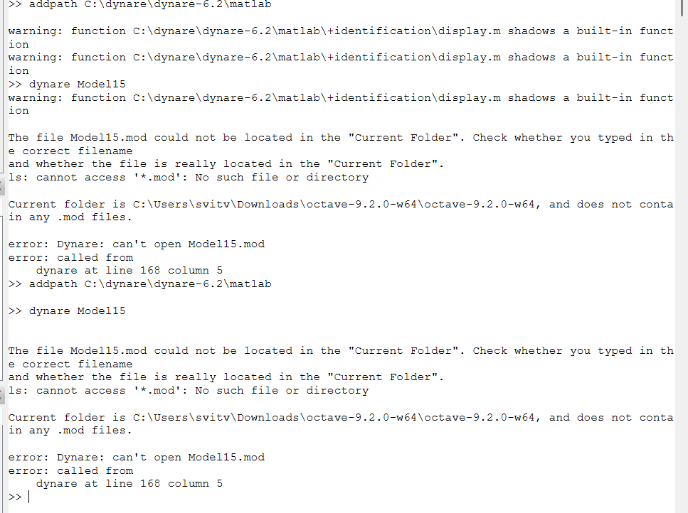
However, I am having a hard time setting a directory, I never had this problem before, could you perhaps give me advice on this please? Here are print screens: