Model with durable good - rank condition ISN'T verified

[paolotardini]

Dear all,

I am trying to write a New Keynesian model with a non-durable and a durable good. The non-durable good features sticky prices; the durable good features flexible prices.

The economy presents a monetary authority that follows a Taylor rule that tracks only inflation for the non-durable good.

I should also add that for simplicity I assume that the depreciation rate of the durable good is zero (delta=0).

I suppose a monetary shock.

Upon running Dynare, I obtain the error message: “There are 4 eigenvalue(s) larger than 1 in modulus
for 5 forward-looking variable(s) The rank condition ISN’T verified!”

Also:

"Error using print_info (line 45)
Blanchard Kahn conditions are not satisfied: indeterminacy

Error in stoch_simul (line 100)
print_info(info, options_.noprint, options_);

Error in RANK_durprod_dgflex (line 330)
info = stoch_simul(var_list_);

Error in dynare (line 235)
evalin(‘base’,fname) ;"

Please find attached the Dynare file with the code of the model.

What mistake am I making? I cannot figure out how to obtain determinacy. Any help would be much appreciated.

Model_durprod_dgflex.mod (7.4 KB)

Please find attached a pdf containing the model’s equations, variables, parameters and steady state variables’ values.

Thesis_model_dg.pdf (230.1 KB)

Thank you,
Paolo

[jpfeifer]

Your first order condition for durables looks strange. How did you derive it? I am puzzled by marginal utility tomorrow not pre-multiplying all of the right side.

[paolotardini]

@jpfeifer,

I retrieve the First Order Condition (FOC) for durables so:

I want to maximize the discounted sum of instantaneous utilities:

U(C_t,K_{t},N_t) = (1-\alpha)\log C_t + \alpha \log (K_{t}) - \frac{(N_t)^{1+\varphi}}{1+\varphi}

subject to the Budget Constraint (BC):

C_t = W_{r,t}N_t -Z_{t+1} +\frac{1+i_{t-1}}{1+\pi_{t}}B_t-v_{C,t}(\omega_{C,t+1}-\omega_{C,t})+ \omega_{C,t}D_{C,t} -q_t[K_{t+1}-(1-\delta)K_t]+\omega_{K,t}D_{K,t}-v_{K,t}(\omega_{K,t+1}-\omega_{K,t})

I substitute C_t with its expression from the BC; I also use the Bellman equation, whereby the maximum of the discounted value of istantantaneous utilities at time t, expressed as \mathcal{W}_t, is:

\mathcal{W}_t= \quad \sup\limits_{X_t^D} U + \beta E_t \left\{ \mathcal{W}_{t+1} \right\}

where X_t^D is the demand for new durable good at time t, namely: X_t^D=K_{t+1}-(1-\delta)K_t.

I apply the Envelope theorem (whereby, roughly, \mathcal{W'}_{t+1}=U'_{t+1}) and take the FOC with respect to X_t^D. Notice that X_t^D determines K_{t+1} and not K_t.

FOC_{X_t^D}: \quad q_t \frac{1-\alpha}{C_t} = \beta E_t\left\{ (1-\delta)(q_{t+1}) \frac{1-\alpha}{C_{t+1}} + \frac{\alpha}{K_{t+1}} \right\}

The expression is so because:

FOC_{X_t^D}: (1-\alpha)\frac{\partial logC_t}{\partial X_t^D} + \beta E_t \left\{ (1-\alpha) \frac{\partial logC_{t+1}}{\partial X_t^D} + \alpha \frac{\partial logK_{t+1}}{\partial X_t^D} \right\} = 0

Notice that:

(1) \quad (1-\alpha)\frac{\partial logC_t}{\partial X_t^D} = (1-\alpha)\frac{\partial logC_t}{\partial C_t}\frac{\partial C_t}{\partial X_t^D}= (1-\alpha) \frac{1}{C_t} q_t;
(2) \quad (1-\alpha)\frac{\partial logC_{t+1}}{\partial X_t^D} = (1-\alpha)\frac{\partial logC_{t+1}}{\partial C_{t+1}}\frac{\partial C_{t+1}}{\partial X_t^D}= - (1-\alpha) \frac{1}{C_{t+1}} q_{t+1}(1-\delta);
(3) \quad \alpha \frac{\partial logK_{t+1}}{\partial X_t^D}= \alpha \frac{1}{K_{t+1}};

Notice also that the BC for C_{t+1} is so:

C_{t+1} = [...] - q_{t+1}[K_{t+2}-(1-\delta)K_{t+1}] = [...] - q_{t+1}[K_{t+2}- (1-\delta)(X_t^D + (1-\delta)K_t]

This is why in (2) I have the expression: \frac{\partial C_{t+1}}{\partial X_t^D}= - q_{t+1}(1-\delta)

I hope everything is clear,
Let me know if you are interested in further clarifications

[paolotardini]

I have corrected the model; now Dynare is running and gives reasonable Impulse Response Functions (IRFs). Here is the updated version of the mod file.

Model_durprod_dgflex.mod (8.5 KB)

I have two questions concerning it. I would be very grateful if you found the time to take a look at them:

1. Do you think I have correctly expressed the inflation for durable goods (dg)? I define it as the ratio between the relative price of dg at time t and the relative price at time t-1, multiplied by the inflation for non-durable goods (ndg) at time t:

1 + \pi_{K,t} = (\frac{q_t}{q_{t-1}})(1 + \pi_{C,t})

where q_t = \frac{P_{K,t}}{P_{C,t}}; \pi_{C,t} is inflation for prices of ndg at time t, namely \frac{P_{C,t}-P_{C,t-1}}{P_{C,t-1}}; P_{K,t} is the level of prices of dg at time t; P_{C,t} is the level prices of ndg at time t.

The expression on the rhs simplifies:
\frac{P_{K,t}}{P_{C,t}} \frac{P_{C,t-1}}{P_{K,t-1}} \left(1 + \frac{P_{C,t}-P_{C,t-1}}{P_{C,t-1}} \right) = \frac{P_{K,t}}{P_{C,t}} \frac{P_{C,t-1}}{P_{K,t-1}} \frac{P_{C,t}}{P_{C,t-1}} = \frac{P_{K,t}}{P_{K,t-1}} = 1 + \frac{P_{K,t}-P_{K,t-1}}{P_{K,t-1}} = 1 + \pi_{K,t}

Computations seem correct to me, but I do not know whether Dynare correctly interprets the expression!

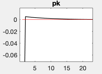
2. The IRF for \pi_{K,t} is strange: the variation is very negative at the beginning, but then one sees small positive and decreasing variations. I interpret this fact so: initially, the level of prices for dg goes below its steady state level (i.e. inflation is very negative), then it slowly increases up to its steady state level (i.e. the inflation is positive, but decreasingly so, until it reaches zero). In other words, the initial decrease in the level of prices is excessive with respect to its steady state level. What do you think of my interpretation? I find it is in line with what says Barsky et al. (2007, Sticky price models and durable goods) at page 6 out of 20 of their pdf file, on the bottom right corner: “Also, while nondurables prices rise slowly, the price of durables overshoots its eventual level.” (they talk about a decrease in the interest rate, while I talk about an increase).

Here is a picture of the IRF for \pi_{K,t} after a positive shock to the interest rate:

Here is the link to the paper I am referring to, by Barksy et al:

https://pubs.aeaweb.org/doi/pdfplus/10.1257/aer.97.3.984

3. Feeding the model I have uploaded to Dynare, are IRFs to be interpreted as absolute variations from the SS or as percentage variations from the SS. I believe IRFs are to be interpreted as absolute variations. What do you think about it?

Thank you,
Paolo

PS Please, also find here the version of the model where all variables are expressed in exp(.), ready for log-linearization. Notice that interest rates and inflation are left in their linear form. All the variable that can be zero in steady state are left in their linear form.

Model_durprod_dgflex_loglin_aut.mod (9.0 KB)

[jpfeifer]

1. Without knowing the model in more detail it is impossible to tell. What you describe sounds sensible, but in the end depends on your numeraire, i.e. in which currency/units you want to express it.
2. Such a behavior is not unusual with jump variables, so I am not too surprised.
3. Yes, your model provides linear deviations. I would not go for a full substitution. See

Question about understanding irfs in dynare

To be more precise: it depends on how the variables in your model are measured. As @stepan-a says, Dynare conducts a linearization. If you for example have a nonlinear model and your model variable is simply the level of output, the IRF will measure the difference between the variable and its steady state (or its mean at higher order). This is the case with https://github.com/DynareTeam/dynare/blob/master/examples/example1.mod In contrast, if your model variable already measures percentage…

[paolotardini]

@jpfeifer,

Thank you so much for your clarification and for always being available.

My numeraire in the economy is the price of non-durable goods, i.e. P_{C,t}. I divide the budget constraint by P_{C,t}, because all nominal variables are expressed in terms of the price of the non-durable good.

Thank you again,
Paolo