Dear Dynare’user,
does anyone know where would go the mark-up shock in the recursive form of the Philips curve such as it is described in SGU(2005) ?
I am trying to do a welfare analysis, and I would like to use estimated shocks from models approximated of first order to calibrate my shocks, but I cannot find a way to get the mark-up shock to produce identical IRFs in both form approximated to the first order ?
Could anyone help ?
Thanks,
Laurent
Markup shocks make the exponent on prices in the FOC for price setting time-varying. This renders a recursive representation impossible and is the reason you only see markup shocks in linearized papers. I would recommend having a look at Justiniano/Primiceri/Tambalotti (2013) who are the only ones I know to consider welfare with markup shocks.
Thank you very much for the reference, that’s a quite interesting one. I haven’t found anything really satisfying myself ( some authors replace it by a dividend shock on first profits…).
I have a related question, my issue is related to the empirical moments obtained when computing conditional welfare which are returned as NaN. I would like to check that most of the policy instruments have a reasonable volatility over my grid and therefore, I need well defined moments for each points on the grid.
Are those moments computed by the Stoch_simul(…, periods=1000) command the conditional variance ?
I am assuming that those are not well defined due to the conditioning set but extending the number of periods to 100000 and burning the first 10000 but that didn’t help, I still got NaN and only the the theorical moments (those returned by the stoch_simul command without the number of periods defined) are well defined. Shouldn’t the two approaches converge to the same moments ? Am I missing something?
I am searching for a way to obtained those unconditional moments without having to run twice Stoch_simul for each point on the grid (one to get the conditional welfare and one for the unconditional moments for this particular set of parameters). Pruning could also help but that might make the measure of welfare problematic (I haven’t found any discussion of welfare ordering and pruning in the literature…).
I am also a bit puzzled about the policy rules computed with moments returned as NaN. Does it make sense with a second order approximation?
Could someone provide help ?
Thanks!
Andreasen (2013) in the EER discusses the issue as well and uses a fixed cost shock to the same effect.
This is most probably an issue with pruning and explosive simulations. That would explain why only only the theoretical moments are well-defined. Pruning should be fine for welfare. See Kim/Kim/Schaumburg/Sims (2008).
You should only need to run stoch_simul once for every parameter draw as all moments should be computed in one run (unless you are trying to mix simulated and theoretical moments)
Hello,
what do you reckon to be the most convenient way to log linearize by hand an equation with time varying exponents, not only in the case of a markup shock as in Justiniano et al. (2013), but also for example in the case of a time varying intertemporal elasticity of substitution in the Euler equation?
Thanks a lot
What do you consider a
?
Something like the Uhlig tricks? I personally always go for a first order Taylor approximation.
Yes, I did it with a first order Taylor expansion too. However, since the derivative with respect to an exponent needs to be multiplied by the log of the base, the effect of the shock changes sign according to whether the ss value of the variable in the base is greater or smaller than one (or it cancels out if it is one). That makes me wonder if it makes sense to consider a shock to an exponent.
Why is that a problem? If you raise a number smaller than 1 to a power, it will become smaller, if it’s bigger than 1 it will increase, if it’s equal to 1, there is no effect.
Can I ask how you linearized the price foc with a time varying markup/elasticity in the exponent? Because there is more than one instances of nominal price with exponent of time varying elasiticites in the exponent and Ln(P_{ss}) comes into the equation (nominal P) but that doesnt have a steady state and I cant figure out how to continue from there. I know there are also nominal prices as denominators such that the whole steady state doesnt blow up but when linearizing the exponent, this wont matter. Ln(P_{ss}) will eventually come into the result. The linearization will have the following term: \epsilon_{ss}Ln(P_{ss})\left(\hat{\epsilon}_{t+s} - \hat{\epsilon}_t \right).
The following is my FOC:
q_t = \frac{\sum_{s=0}^{\infty} (\beta \theta)^s \Lambda_{t+s,t}\epsilon_{t+s}\phi_{t+s} (\Pi_{ss}^{s\iota}\Pi^{1-\iota}_{t+s-1,t-1})^{-\epsilon_{t+s}}\frac{P_{t+s}^{\epsilon_{t+s}}}{P_t^{\epsilon_t}}y_{t+s}}{\sum_{s=0}^{\infty} (\beta \theta)^s \Lambda_{t+s,t}(\epsilon_{t+s}-1) (\Pi_{ss}^{s\iota}\Pi^{1-\iota}_{t+s-1,t-1})^{1-\epsilon_{t+s}}\Pi_{t+s,t}^{-1}\frac{P_{t+s}^{\epsilon_{t+s}}}{P_t^{\epsilon_t}}y_{t+s}}
I’m quite sure about the math. I have checked it with Eric Sim’s notes. Also the nonlinear recursive form gives correct results in my dynare code. The difference from Eric Sim’s notes is that the firms which cannot change their price, set it based on an index of steady state inflation and past period’s inflation. The numerator and denominator have been divided by P_t^{\epsilon_t} so that the steady states of both the denominator and the numerator are finite. If you set the elasticity as constant, it will yield the foc we are familiar with. If you consider the prices as compeltely non-sticky (s=0) it will yield the familiar markup equation q_t = \frac{\epsilon_t}{\epsilon_t-1}\phi_t.
The term \epsilon_{ss}Ln(P_{ss})\left(\hat{\epsilon}_{t+s} - \hat{\epsilon}_t \right) that I previously said will emerge in linearization comes from the fraction \frac{P_{t+s}^{\epsilon_{t+s}}}{P_t^{\epsilon_t}} that is present in both numerator and denominator. I am most probably linearizing wrong and will appreciate if anyone can help.
This issue still remains if we remove the inflation indexation feature and use the typical Calvo type price foc. I also checked other sources and am sure of the written foc. So the only problem that remains is that how we linearize it. I just do not understand how authors like Smets and Wouters (2007), Tambalotti, Primiceri, and Justiniano (2013), and Christiano, Motto, and Rostagno (2014) linearize a Cavlo-driven price foc with variable markup in their respective papers. The most detailed paper of the three in regards to the linearization appears to be Smets and Wouters (2007) but even they refrain from explaining exactly how they reach the reported final linearized equation, as they use a function “G” for their kimball aggregator for the nonlinear foc and do not expand on how they reach the final linearized equation (the variable parameter \epsilon_{p,t} is inside that function in their paper).
I was able to locate an old detailed derivation for wage markup shocks. Maybe that can help. In that derivation, it’s the ratio of prices that shows up everywhere.
Wage_Markup_Linearization.pdf (148.4 KB)
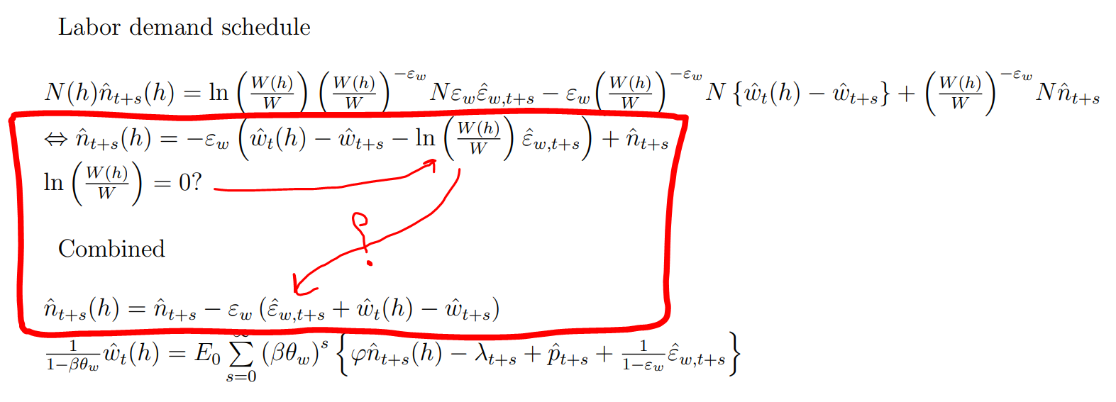
Thank you for providing the material. I dont understand the following from the pdf you attached.
Should \hat{\varepsilon}_{w,t+s} be removed?
Also, the following
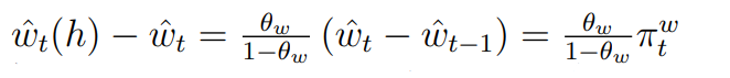
It seems to imply \frac{w_t(h)}{w_t} = \left(\frac{w_t}{w_{t-1}}\right)^{\frac{\theta_w}{1-\theta_w}} which I dont know where it originates from.
Thank you in advance.
I did not write this PDF, so I don’t know what is going on here. The first part indeed looks like a mistake.
The second one looks as if the Calvo law of motion was used, but I am not sure.