My identification anaysis shows “WARNING: Komunjer and Ng (2011) failed”, and is it ok to ignore this one?
I have 5 observed variables which include y( real gdp per capita), c(real consumption per capita), i(real investment capita), r(nominal rate) and pi(inflation rate). When I used all of them to run estimations, I found that the likehood was weird but the identification seemed fine.
I don’t know where I got wrong, the priors? or my data treatment. I think I strictly followed instructions of Dr. Pfeifer’s paper to process my data which was that firstly, taking the logarithm of data(already seasonal adjusted), secondly using One-sided HP filter and finally taking out the mean. My model is linearized and all observed variables followed this procedure. If anything and anywhere is wrong please correct me. And what can I do to fix this issue?
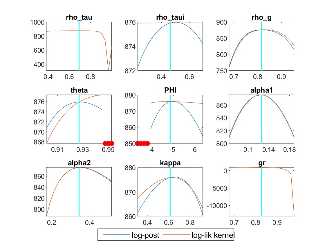
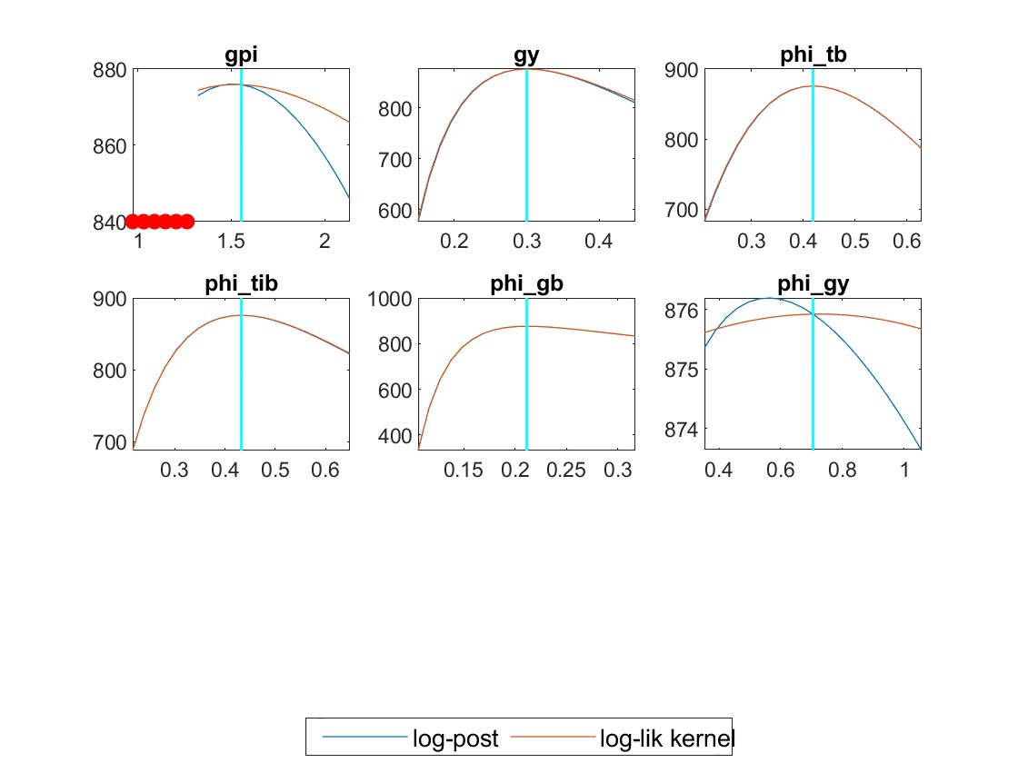
My mode check plots have many red dots. Is there any solution?
Yes, if the other identification checks do not flag issues you can ignore the warning.
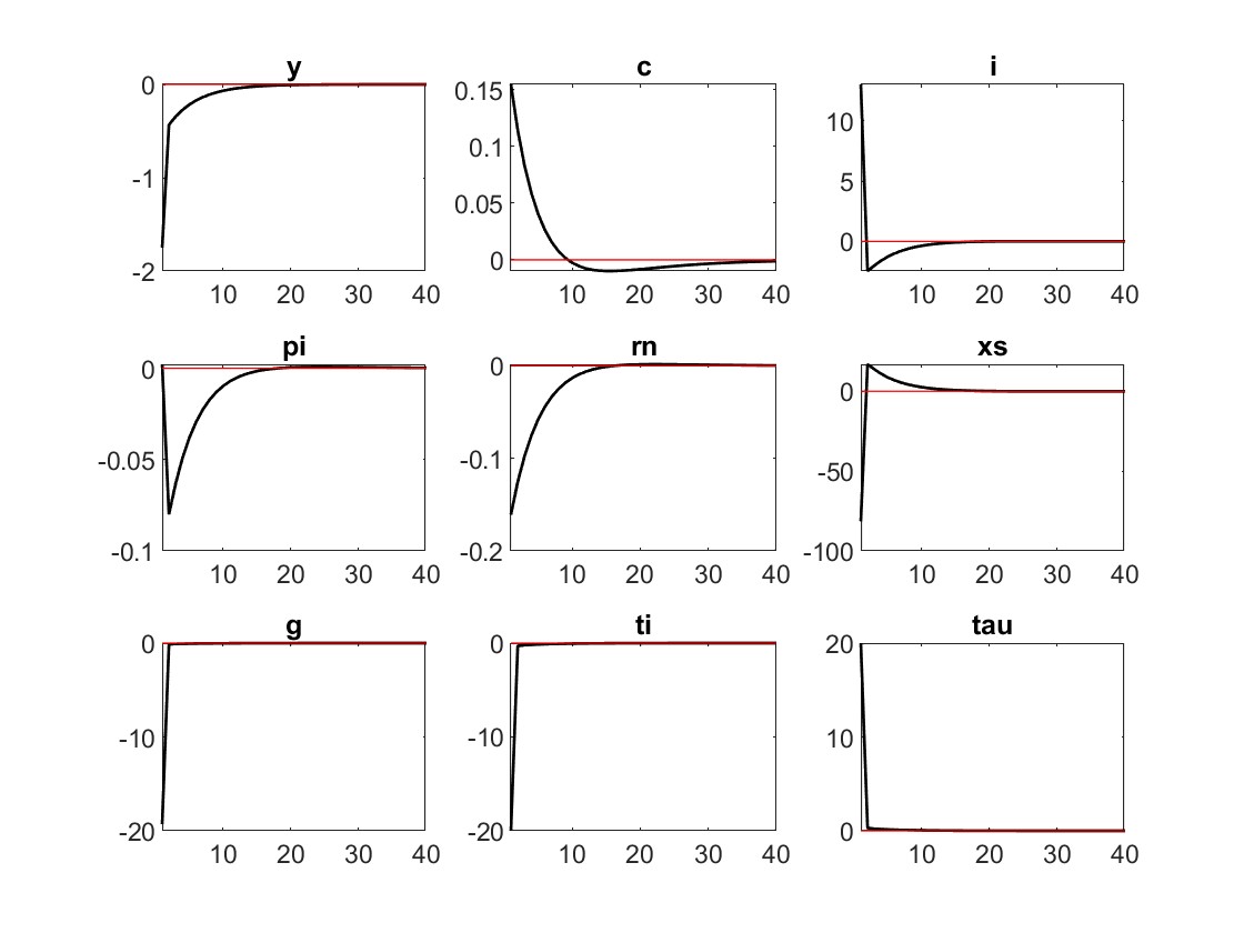
Those differential values for the likelihood when dropping r suggest that something in the mapping from model to data went wrong. It looks to me as if drn in the data is way too volatile. You calibrate the shocks to have a rather high standard deviation, but
Your model runs into the indeterminacy region. That may be related to the problems in 2.
Fix the other issues, then try again. Try using mode_compute=5 for faster results and better diagnostics.
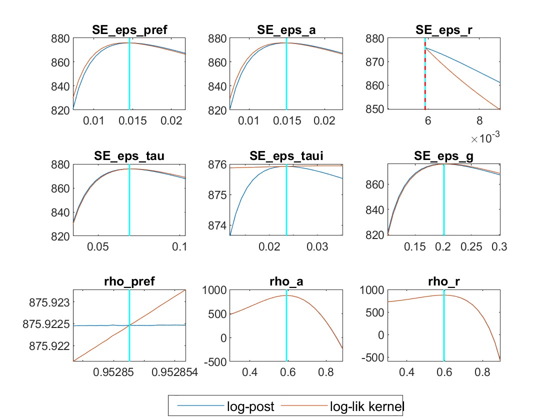
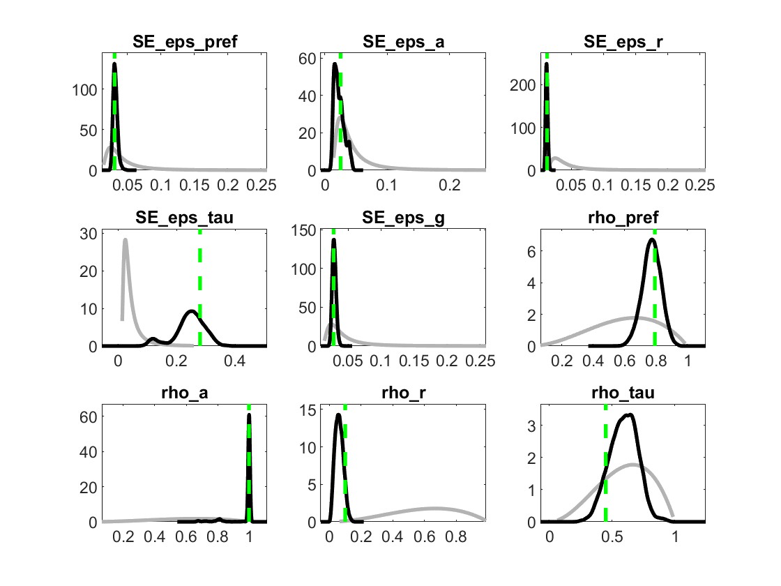
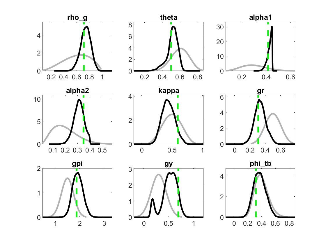
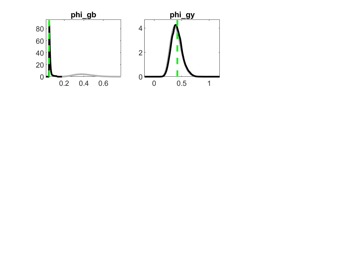
But still, some parameters like rho_pref, phi_gy and rho_tau, their plots are unusual.
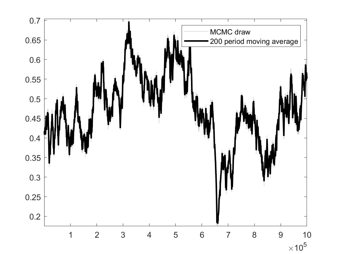
2.And traceplots almost remian unchanged. What could explain such traceplot behavior?
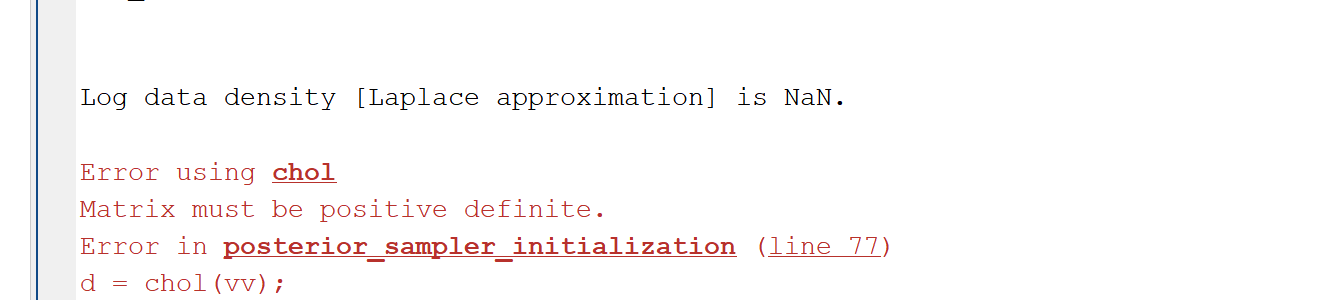
I tried mode_compute=5 but another problem emerged:
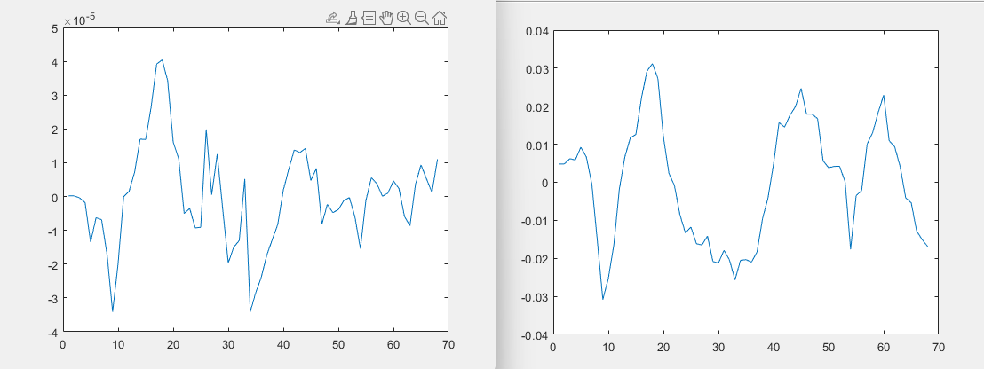
Are you sure the observation equations are correct? Why does the interest rate rn move in the range of 10e-5 only, while inflation dpi is three magnitudes larger:
Only you can answer that. They look more conformable now, but there is only one correct mapping from model to data. I don’t know whether you have found it.
Shouldn’t it be increased or is my model setting wrong?
If the negative impact of Y and PI both are bigger than rm , I think rn is supposed to increase at first and then decrease instead of decreasing immediately. Does my understanding sound correct?
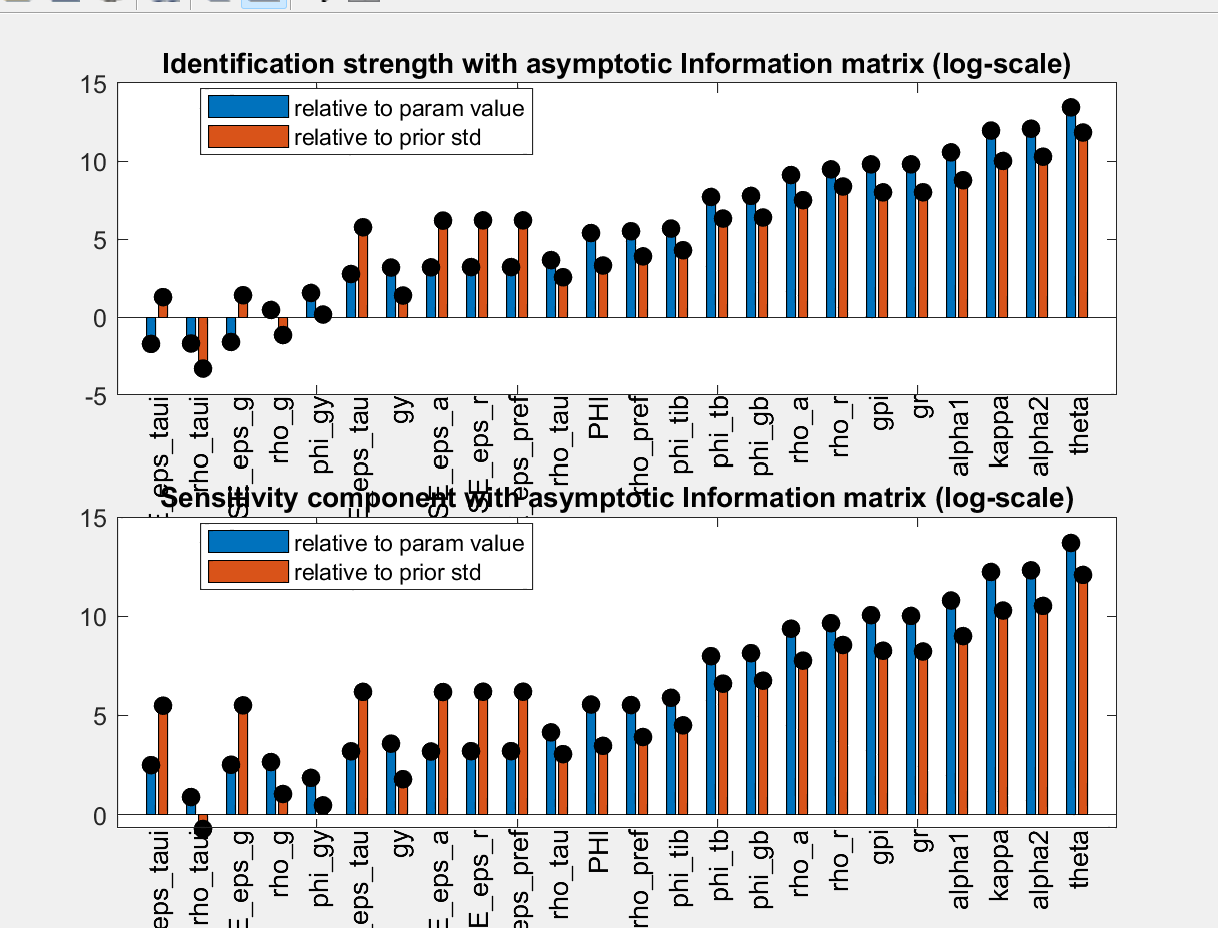
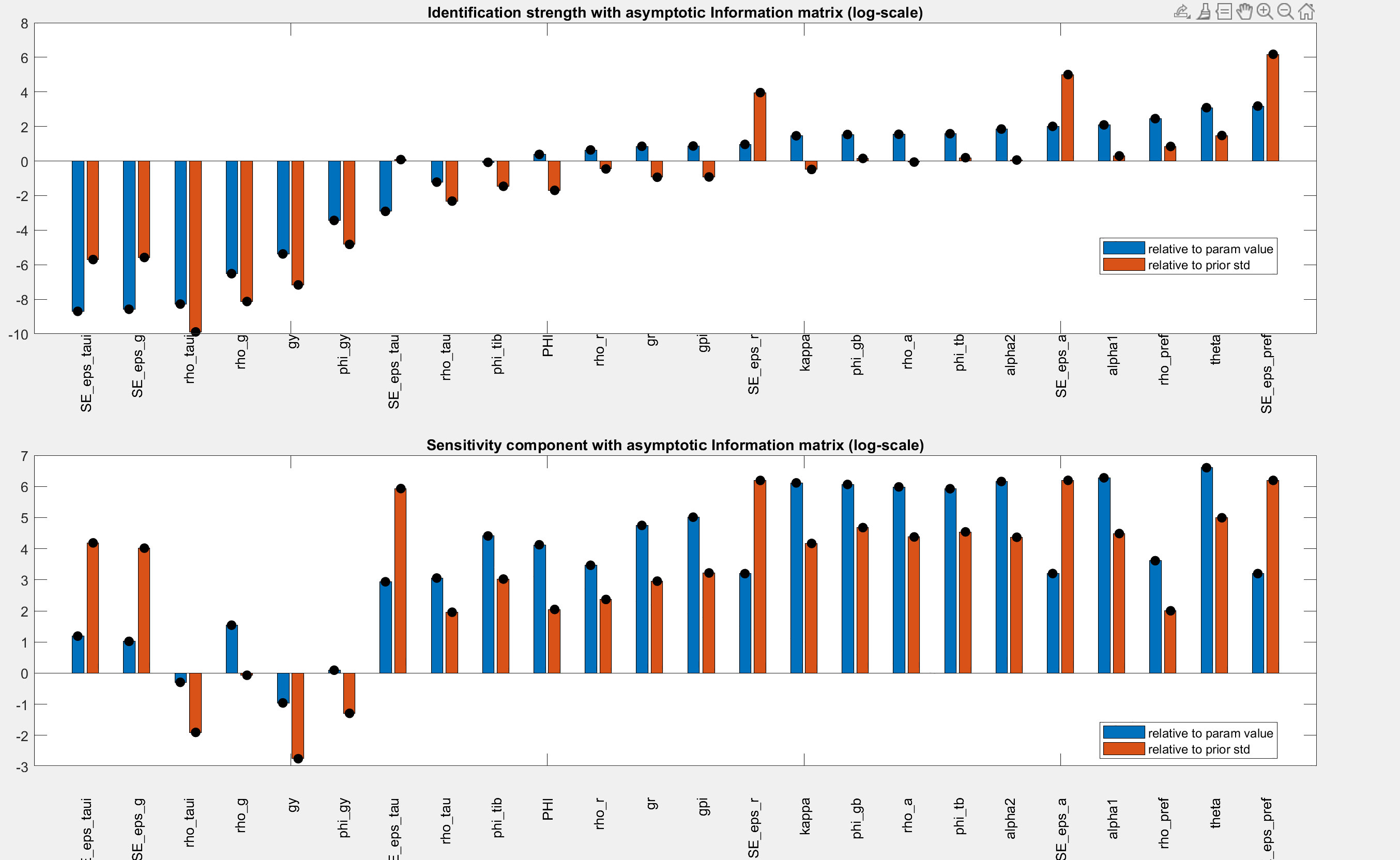
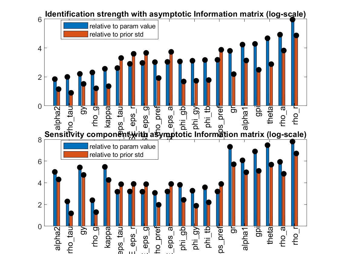
The parameters are weakly identified. Despite trying multiple times, I have been unable to achieve stronger identification. Should I still proceed with these results?
My estimation results indicate that rho_r is below 0.1. This suggests that my model predicts an extremely short-lived impact of a monetary policy shock, which seems unrealistic. How can I identify where the issues lie?
I don’t find that too unusual. What are monetary policy shocks? If you think about them as policy mistakes, i.e., temporary deviations from the monetary policy rule, they should not be autocorrelated, i.e. predictable.
.
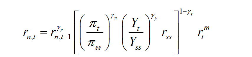
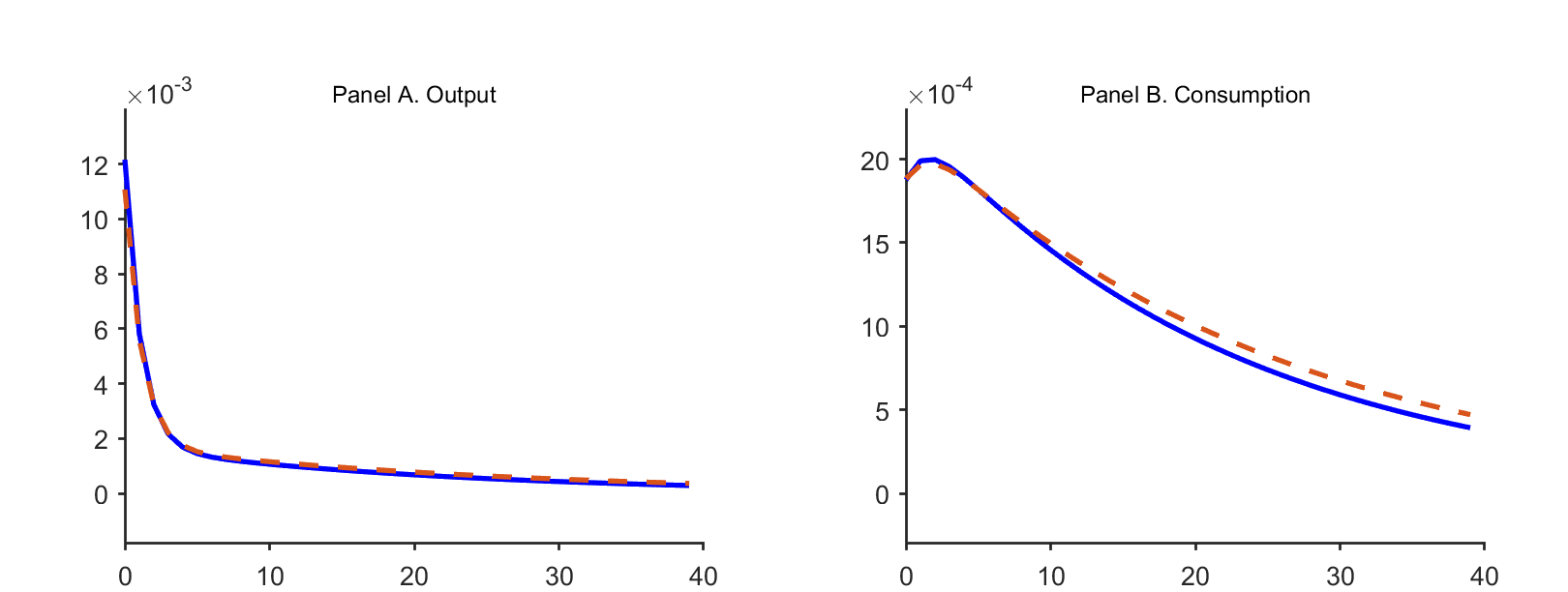
The order of magnitude of the y-axis is very small. If I want to magnify it by 100 times, should I magnify it directly during the plotting process or should I magnify the model by 100 times?
I notice that some authors magnify the data by 100 times, except for the interest rate. If I have to magnify the model by 100 times, I should magnify both the measurement equations and the data, right? Therefore, my measurement equations change to dy = 100*y . But what about the equation for the interest rate? Does that also need to be multiplied by 100?
Which of these methods is correct? I simply aim to enhance the readability of the figures and unify the order of magnitude.
Usually, it is safest to scale the IRFs for plotting, not the data. For example, if your log output deviation shows a value of 0.001, the mean 0.1 percent. and you would represent it in the plots at 0.1 and outline that the graph is in percent.
I am currently encountering another issue.
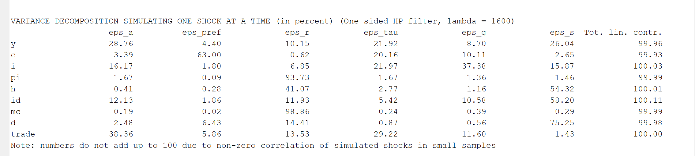
The sum of the numbers in the shock decomposition does not equal 100. In your previous response, you suggested using theoretical moments when periods=0 . However, I would like to know whether, if I insist on using simulated moments, I need to provide an explanation for why the sum of those numbers does not equal 100. Additionally, regarding the one-sided HP filter option, should I employ it? This is because I prefer the results obtained when the HP filter is applied.
Thank you very much for your reply, I have understood now — both the model and the data need to be processed in the same way.
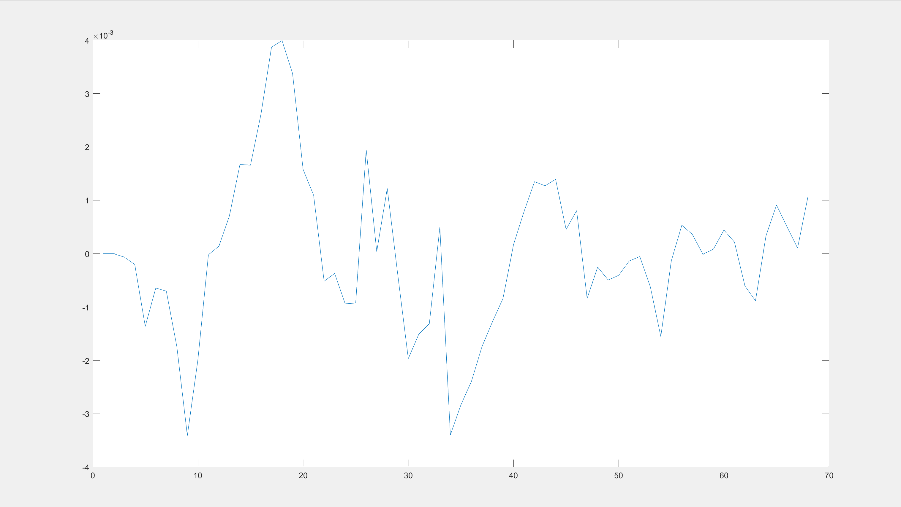
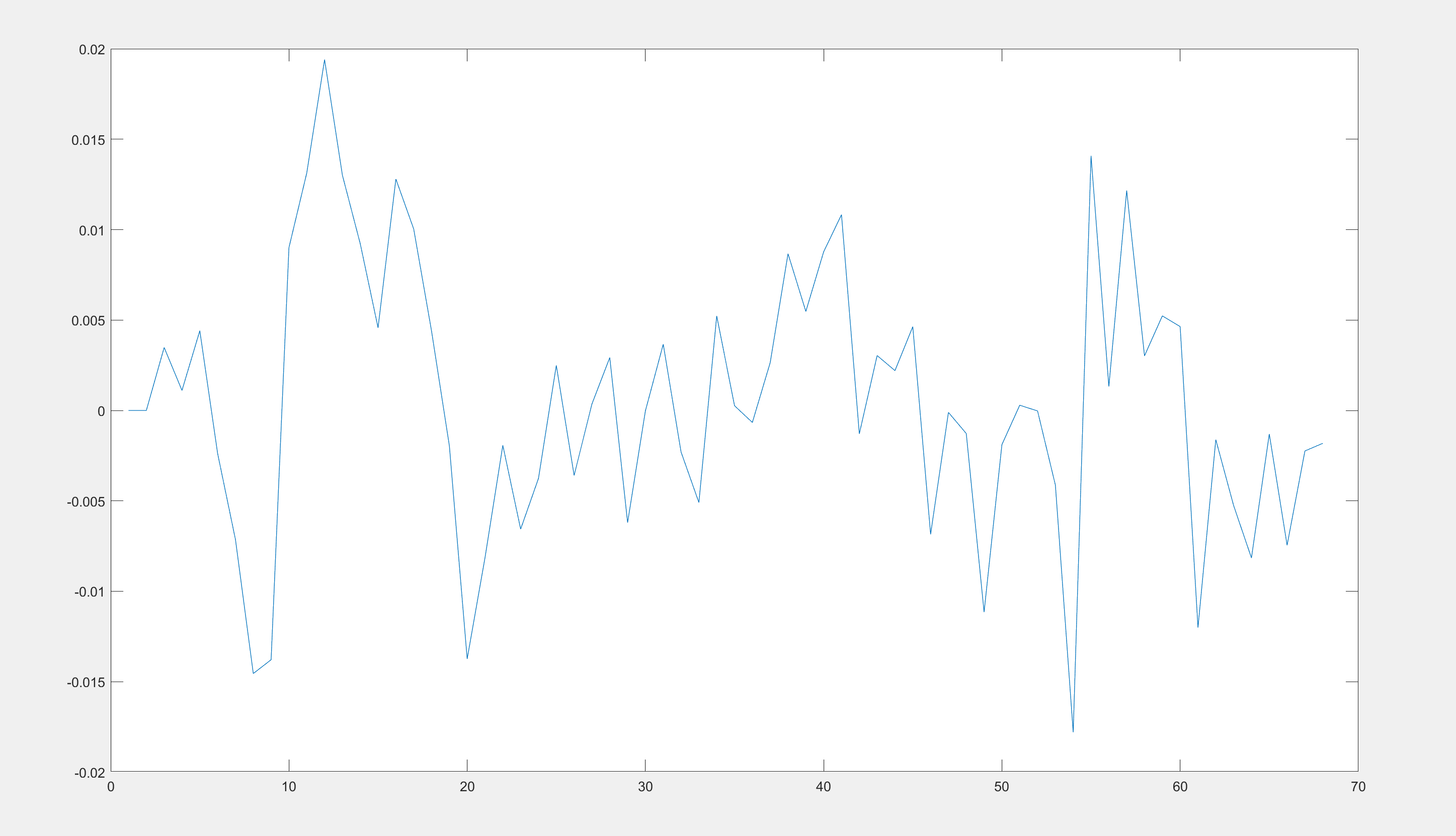
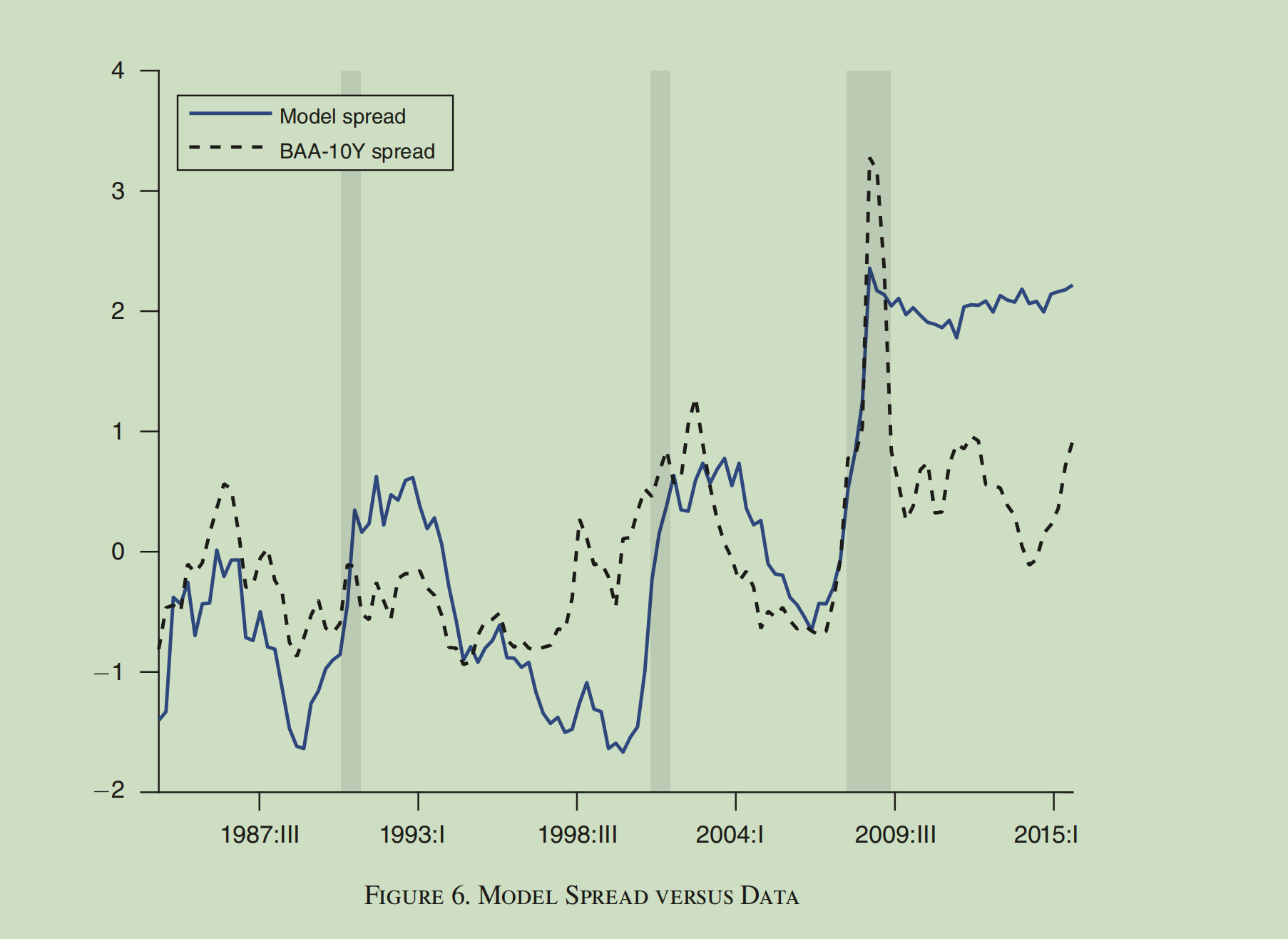
I now wish to compare the model variables with actual data, as shown in the figure below.
I am not sure how to achieve that. Which data stored in oo_ should I use?