I’m currently working on a model I referred to in a previous post on the forum.
I’m having trouble understanding the behavior of debt in my model. Assuming both worker types have similar productivity initially, an increase in one group’s labor force should lead to borrowing/lending between households.
Since agents choose B_t2(+1) today, I need the adjustment to occur with a one-period delay. Is this behavior standard in Dynare? If not, how should I define debt to capture that timing?
means that B_t2 is not predetermined. To make B_t2 predetermined, it would need to be shifted by one period. Put differently, B_t2(-1) would be predetermined, while B_t2 is the value chosen today.
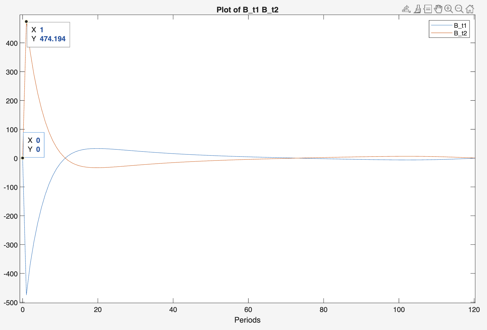
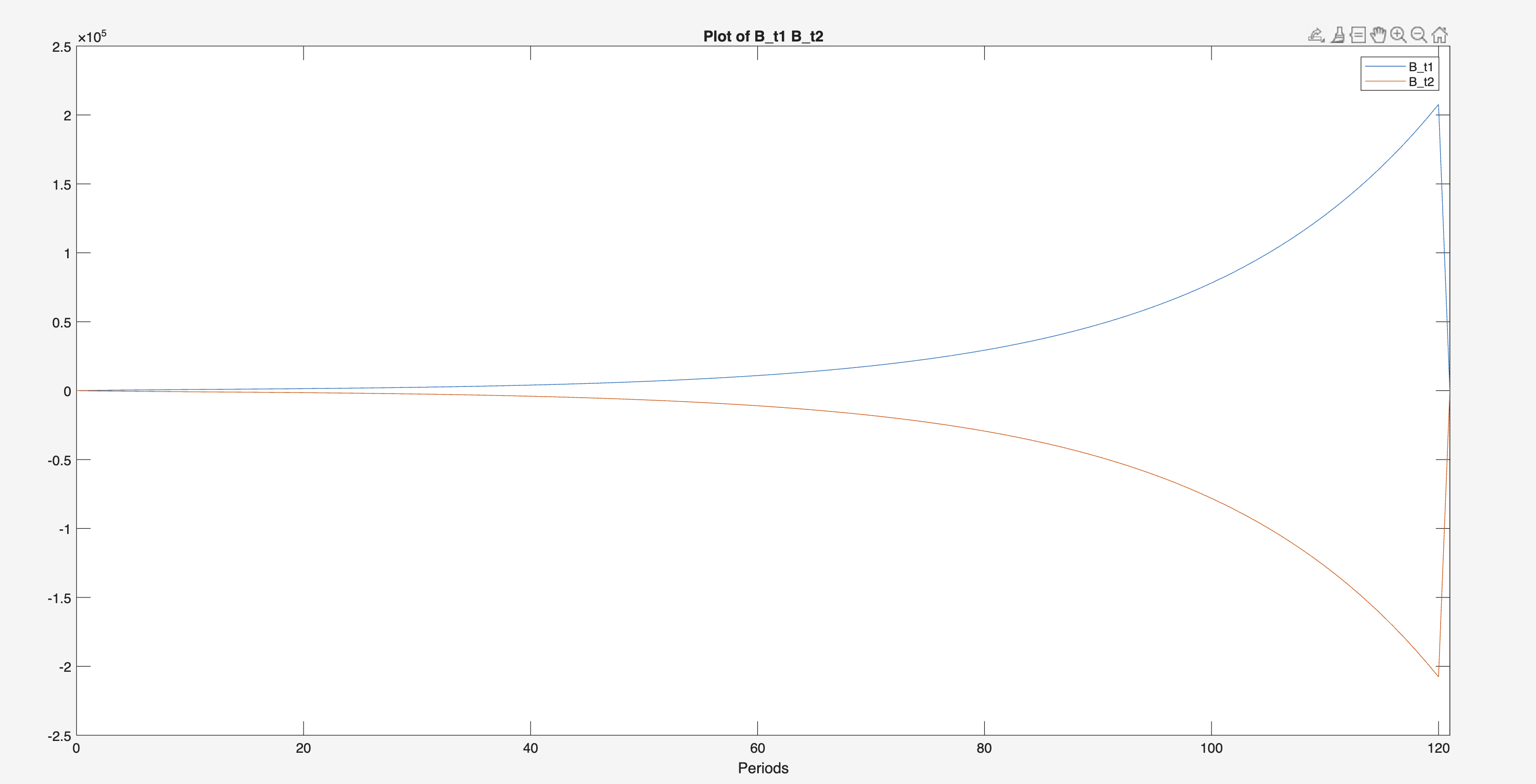
But that leads to an even stranger result. If you look at the attached image, you’ll see that debt stays around zero for most of the transition path and then suddenly drops at the final period. That behavior doesn’t make much economic sense to me.
I was wondering: was your suggestion also implying that I might need to revise the timing of other variables as well? For example, the interest rate i is defined at +1 in the Euler equation—could that be a source of inconsistency here?
The other files are the same ones I used in my original post.
What I’ve been reading is that when using perfect foresight and having a finite time horizon, there is no optimal path for repaying debt. As a result, the solver determines that the simplier course of action is to accumulate debt until period T-1 and pay the interest in the final period. That dynamic doesn’t seem very reasonable to me.
I read that adding a rising cost to indebtedness could correct this, but I’d prefer not to impose additional conditions.
Not a specific paper or forum post, no. It’s something I’ve inferred through iterations with different LLMs and from the behavior I’ve observed in Dynare while running my model, as well as simpler versions of it, where the same debt path dynamics appeared.
I’m still trying to resolve this issue, and I wanted to explore whether the behavior of debt remains consistent in the context of a stochastic simulation. I did this assuming that the labor force shock follows an AR(1) process.
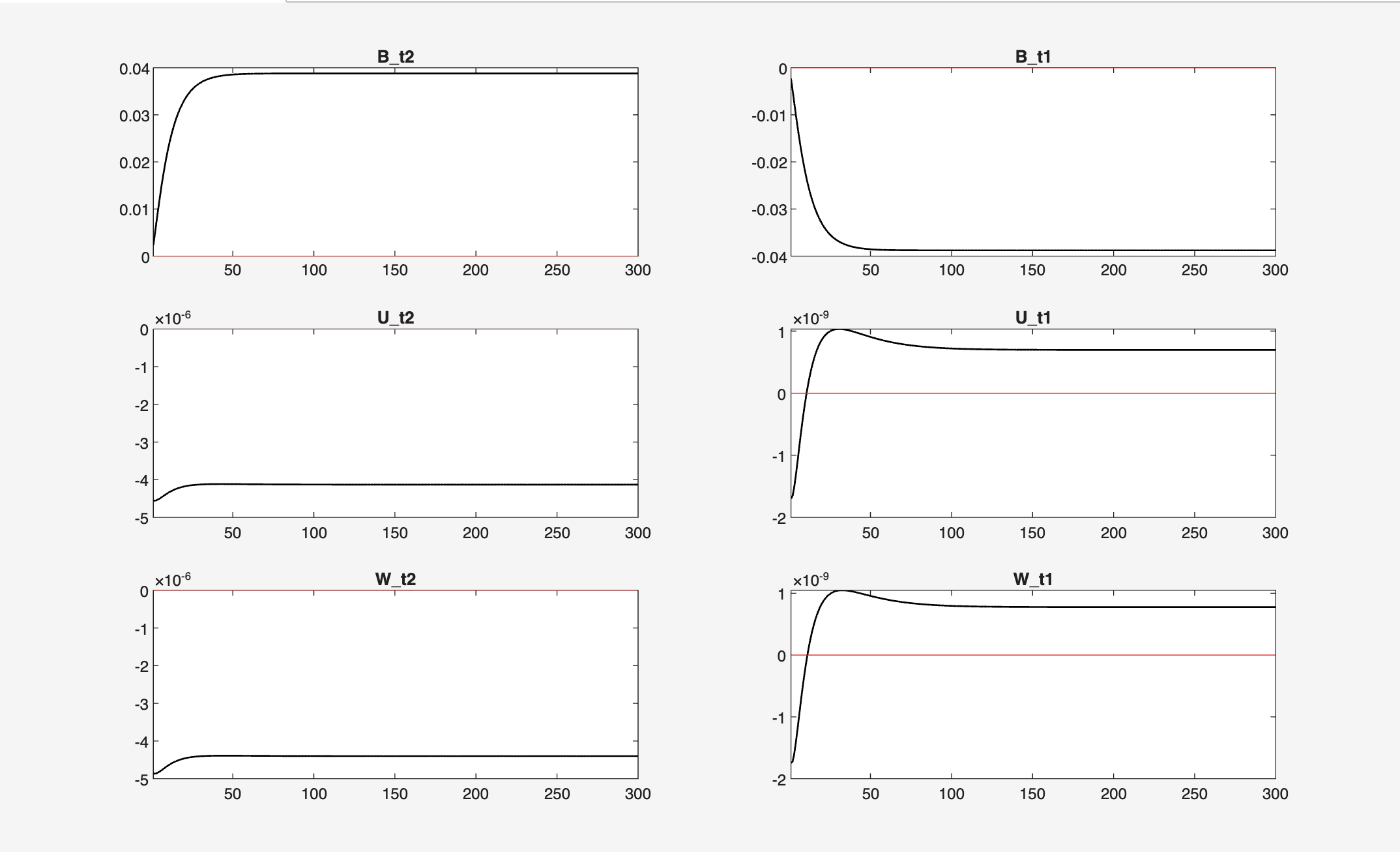
What I find puzzling is that, in this type of setting (stochastic simulation), where all variables are supposed to return to their original steady state, the debt variable—along with those representing the present value of unemployment (U_t1, U_t2), employment (W_t1, W_t2), and debt itself (B_t1, B_t2)—do not return to steady state.
I would like to know whether this implies that the IRF simulation is correct and that such behavior can occur in these settings, or if it instead suggests a problem with the simulation.
I’ve attached the updated code files for your reference.