ZLB, Optimal policy, Welfare

[Andy_zhao]

Hi all,

I have some questions and look for helps, regarding optimal monetary policy at ZLB solving with perfect foresight in Dynare 4.6

I have a textbook New Keynesian model with short-term nominal interest rate being constrained by the ZLB. I am doing optimal monetary policy under the assumption of perfect foresight as in Gali(2015) chapter 5. One departure from the dynare code programmed by Professor Pfeifer’s code for Gali(2015) chapter 5 is that I assume an AR(1) preference shock following Jung, Teranishi and Watanabe (2005). I have several puzzling issues:

1, The dynare command “ramsey_constraints” and “ramsey_model” in combination produces the solution of optimal commitment policy at ZLB with perfect foresight. I am wondering are there some similar dynare command that can also be applied directly to solve optimal discretionary policy at ZLB with perfect foresight. I have tried to use the command “ramsey_constraints” and “discretionary_policy”, it does not seem to work. Does that mean I have to first derive manually the first-order condition (with Kuhn-Tucker condition associated with the inequality constrain) of optimal discretionary policy at ZLB and put those first-order conditions into dynare?

2, How can I compute the implied (conditional or unconditional) welfare under optimal monetary (commitment or discretionary) policy at ZLB when solving with perfect foresight?

Thanks a lot in advance!

Warm regards
Andy

[jpfeifer]

1. You cannot do discretionary policy with occasionally binding constraints in Dynare. The discretionary_policy is for stochastic models and is also not compatible with ramsey_constraints.
2. Please upgrade to 5.0 and use the evaluate_planner_objective-function.

[Andy_zhao]

Dear Johannes,

Thank you so much for your kind reply. This is really helpful! Now, I understand that to study optimal discretionary policy at ZLB with perfect foresight shocks, we do need to derive manually the first-order condition as you did for Gali(2015) chapter 5. Would it be possible for me to have a few follow-up questions：

1, I have upgraded dynare to version 5.0. As you suggested, I tried the “evaluate_planner_objective”-function in the code you did for Gali(2015) chapter 5 Gali_2015_chapter_5_discretion_ZLB.mod (6.3 KB) and Gali_2015_chapter_5_commitment_ZLB.mod (5.5 KB). It seems that to use “evaluate_planner_objective” function, the commond “planner_objective” is required beforehand. However, when I do that, Dynare reports mistakes saying “the “ planner_objective ” command must be used with a ramsey_model, a ramsey_policy or a discretionary_policy statement and vice versa ”. My question is, if we already put the first-order conditions associated with optimal policy at ZLB into dynare, as you did you for Gali(2015) chapter 5, how can we apply the “evaluate_planner_objective”-function?

More specifically, based on your code Gali_2015_chapter_5_discretion_ZLB.mod (6.3 KB) and Gali_2015_chapter_5_commitment_ZLB.mod (5.5 KB), suppose I want to compute the welfare associated with the model-consistent loss function, which is (pi^2 + vartheta*x^2), Could we make it? How should we apply the “evaluate_planner_objective”-function?

2, Further, suppose I want to compute the (conditional or unconditional) variances of inflation “pi” and output gap “x”, under optimal discretionary policy at ZLB with perfect foresight shocks. Can we do that? My question is how could we obtain (conditional or unconditional) second moment of inflation “pi” and output gap “x”, based on your code Gali_2015_chapter_5_discretion_ZLB.mod (6.3 KB) and Gali_2015_chapter_5_commitment_ZLB.mod (5.5 KB).
.

Thanks for your time. You help is highly appreciated!

Best regards
Andy

[jpfeifer]

The evaluate_planner_objective-function is only for cases where Dynare computes the planner FOCs. If you compute the FOCs yourself, you can include the recursive definition of the planner objective in the model-block.
In your questions there is a conflict between perfect foresight and using a welfare criterion derived based on variances. With perfect foresight, that will not work as these variances are generally zero. Rather, you usually consider the simulated ex-ante welfare.

[Andy_zhao]

Dear Johannes,

Sorry for the late reply. I really appreciate your help! Would you mind if I have few follow-up questions:

1, As you said, “ If you compute the FOCs yourself, you can include the recursive definition of the planner objective in the model-block.” and “there is a conflict between perfect foresight and using a welfare criterion derived based on variances”. I am not sure if I understand it correctly. From my understanding of your explanation, adding the recursive definition of welfare into the mode_block to obtain correct welfare is only possible when shocks are assumed to be stochastic and we use “stoch_simul” command to simulate the model stochastically. However, in the environment of perfect foresight, even adding the recursive definition of welfare in the model_block would lead to a zero value of welfare as the variances of inflation and output gap are generally zero. Am I right?

2, Now I have two mode files and both can replicate Jung, Teranishi and Watanabe (2005), which is essentially optimal commitment policy for the textbook NK model under ZLB and AR(1) perfect foresight demand shock.

Jung2005_Occbinding.mod (2.1 KB) let Dynare to compute the FOCs. I use the
“evaluate_planner_objective” function there. If we run it, Dynare reports the values of welfare:

Simulated value of unconditional welfare: 0.00000000
Simulated value of conditional welfare: 0.00146289

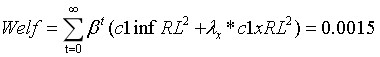
Jung2005.mod (2.4 KB) is also the code to replicate Jung, Teranishi and Watanabe (2005). But now I derive the FOCs manually and puts FOCs into Dynare directly. Also, as you suggested, I add the recursive definition of welfare: “Welf = (c1infRL^2 + lambda_x * c1xRL^2) + bettap * Welf(+1)”, where the period loss function is ”L_t = (c1infRL^2 + lambda_x * c1xRL^2)” with “c1infRL” being inflation and “c1xRL” being output gap. If we run Jung2005.mod (2.4 KB), it also reports the values of “Welf”, which consists of sequence of numbers (if we choose the first ten periods):

Welf = [ 0 0.0015 0.0006 0.0005 0.0003 0.0001 0.0000 0.0000 0.0000 0.0000 ]

My question is what might be the differences and links between the welfare reported from Jung2005_Occbinding.mod (2.1 KB) and the “Welf” generated from Jung2005.mod (2.4 KB).

3, A follow-up question is how does Dynare compute the welfare if we let Dynare compute the planner’s FOCs and apply the “evaluate_planner_objective-function” under perfect foresight shock, for example for Jung2005_Occbinding.mod (2.1 KB).

4, Would it be possible for you to talk more about “simulated ex-ante welfare”? What does that mean? How does it differ conceptually with the welfare number obtain from runningJung2005_Occbinding.mod (2.1 KB) or Jung2005.mod (2.4 KB)? How should we think about the difference between “simulated ex-ante welfare” under perfect foregisht shocks and the (conditional or unconditional) welfare we typically use under stochastic shocks? And how should we compute it in Dynare, or alternatively how to compute it for Jung2005.mod (2.4 KB)?

5, In case of stochastic shocks, we can use the conditional or unconditional welfare to evaluate the performance of different policies. My question is what is the proper or best measure of welfare in models with ZLB and perfect foresight shock?

Thanks a lot in advance!

Best regards
Andy

[jpfeifer]

1. The reason you get variances in most objective functions is considering unconditional welfare and therefore taking unconditional expectations of squared deviations from steady state. But that does not work for perfect foresight because here you are not working with unconditional expectations. In fact, your information set is exactly specified.

2. With perfect foresight, there is no point in approximating the household objective function in terms of variances/gaps. Rather, once you have computed the solution for consumption and labor, you can immediately compute the path for welfare based on the utility function.

3. What Dynare reports for

   Simulated value of unconditional welfare: 0.00000000

   is the value of the objective function in the terminal steady state. The one for

   Simulated value of conditional welfare: 0.00146289

   is the value of the objective function in the initial simulation period. It is the Welf- value in the second entry (which is the first simulation period due to ? M_.maximum_lag=1)

[Andy_zhao]

Dear Johannes,

Thank you so much for your detailed and clear explanation. This really help me a lot!

(a), Now I see that, under perfect foresight shocks, all the information is fully known to all agents in the model without any uncertainty, and hence the model is purely deterministic. So unconditional expectations of square deviation of model variables from steady steady would be zero, implying a zero value of unconditional welfare, as reported “Simulated value of unconditional welfare: 0.00000000 ”.

The conditional welfare under perfect foresight shock can be computed out directly, and simply given by the discounted square sum of the paths of inflation and output gap (in deviation from their steady state) conditional on the deterministic perfect foresight natural rate shock. The “Simulated value of conditional welfare: 0.00146289” in the first case exactly coincide with the value of “Welf” at the initial simulation period in the second case which is given by,

if we plug into the implied path of “c1infRL” and “c1xRL” conditional on the perfect foresight shock.

(b), It seems we can also use “extended_path” to obtain the simulated value of variance of model endogenous variables, which can further be employed to compute the welfare. I am not sure whether it makes sense or not, and is it the “simulated ex-ante welfare” you mentioned earlier?

Jung2005_commitment_FOC_extendpath.mod (2.6 KB) is equipped with Dynare the FOCs of the optimal commitment policy for the textbook NK model under ZLB and AR(1) perfect foresight demand shock. Now I add the “extended_path(periods=10000,lmmcp)” at very end of the mod file. After running the mod file, “oo_.exo_simul” provides the simulated value of the innovation of the shock. “oo_.endo_simul” gives us the simulated long series of model variables. We can then compute second moments based on the simulated series in “oo_.endo_simul”, and further compute the welfare in making use of the quadratic loss function ”L_t = (c1infRL^2 + lambda_x * c1xRL^2)”.

My questions are:

(1), Is point (b) a reasonable measure of welfare under perfect foresight. Is the way of computing welfare in point (b) consistent with the “simulated ex-ante welfare”?

(2), If so, would it possible for you to comment on which welfare measure make more sense in evaluating the performance of different polices: the conditional welfare (“Welf” at the initial simulation period) in point (a) or simulated welfare in point (b)?

Thanks for your time!

Best regards
Andy

[jpfeifer]

1. I am not sure why you would want to go for extended_path. Didn’t you already get what you need with perfect_ foresight?
2. See

An elementary question on SGU 2006 expanded version

The answer always depends on what you are trying to do. Conditional welfare is something used when you ask whether a change in a policy regime is beneficial. In that case, you would start at or somewhere close to the steady state of the old regime and this is the starting point for the implementation of the new policy. If the steady states in the new regime is different, then you would need to compare welfare at the steady state of the old regime. Unconditional welfare in contrast is not concer…

[Andy_zhao]

Dear Johannes,

You are totally right! I already get the conditional welfare with perfect_foresight, which is exactly what I need.

Thank you so much for your time and help! Wish you have a great weekend!

Best regards
Andy