Dear Professor Pfeifer:
I am estimating the parameters of DSGE model shocks. However, the posterior mean of one parameter (epsilon) is exactly the same as its prior mean, while the others look quite normal.
part of the estimation results is:
ESTIMATION RESULTS
Log data density is -490.260552.
parameters
prior mean post. mean 90% HPD interval prior pstdev
epsilon 0.900 0.9000 0.9000 0.9000 beta 0.0250
alphaP 0.500 0.5061 0.4736 0.5366 beta 0.0500
kappaK 1.000 0.8178 0.7815 0.8566 gamm 0.1000
kappaB 1.000 1.1786 1.1132 1.2601 gamm 0.1000
The epsilon is the external habit persistence parameter, as in Iacoviello and Neri (2010)'s households. I tried another calibrated value (and estimation prior) but the posterior mean is still exactly the same as its prior.
ESTIMATION RESULTS
Log data density is -317.192177.
parameters
prior mean post. mean 90% HPD interval prior pstdev
epsilon 0.800 0.8000 0.8000 0.8000 beta 0.0250
alphaP 0.500 0.5522 0.5454 0.5569 beta 0.0500
kappaK 1.000 0.6587 0.5864 0.7302 gamm 0.1000
kappaB 1.000 1.2153 1.1510 1.2805 gamm 0.1000
The stoch_simul version works well and I use estimated_params_init(use_calibration). Why could this happen? Thanks in advance.
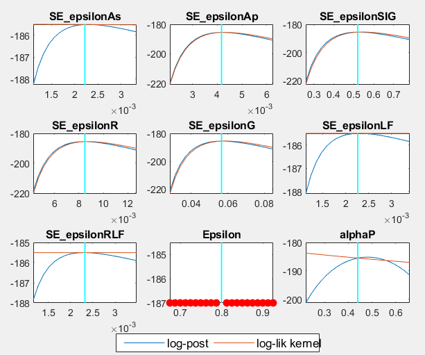
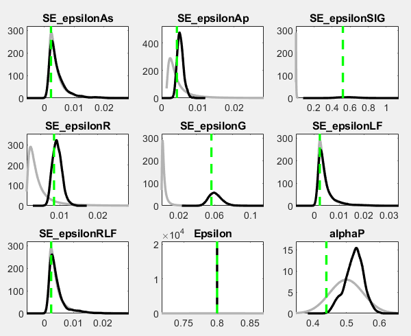
You should investigate the mode_check and prior-posterior plots.
Thanks for your reply, dear professor. I used nodisplay in stoch_simul block and it also worked in estimation blok, thus I didn’t see the plots directly last time. And now I post my figs here. Big red dots appear everywhere expect for the chosen prior value. I know Big red dots indicate parameter values for which the model could not be solved due to e.g. violations of the Blanchard-Kahn conditions in your Introduction-to-Dynare-Graphs handouts. Since stoch_simul works well and its irfs look quite normal, I think there is no BK condition problem. I wonder how could this happen?
It seems you are hardcoding your steady state values instead of adjusting the steady state when the parameters change. That should explain the red dots for Epsilon.
Thanks for the reply, professor. That really sounds like the problem. I use the steady-state-value-targeted strategy and calibrate some steady-state-ratio relationships instead of parameters. I used to be a little confused because I thought it wouldn’t happen to parameters like external habit persistence.
And one more question, is it acceptable if I have 8 shocks but only 4 observables in the estimation? I mean if this will be argued since I quit the chance of adding more information from data. More observables always cause a log density of -inf and I can only delete some because there is always potential linear relationships that I can hardly find when adding a new observable.
I think now I’ve caught the point on this issue. Thank you so much professor, your reply is helpful as usual.