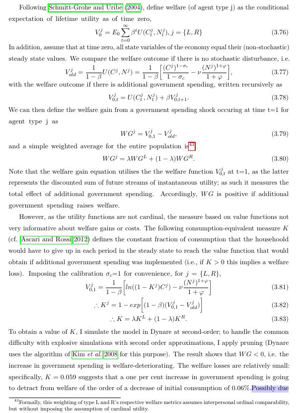
I am working with a medium-scale two-agent New Keynesian model with government spending and want to analyse the welfare effects of a 1% increase in fiscal spending using the methodology set out in Schmitt-Grohe and Uribe (2004). The approach I’m using is summarised below and the associated Dynare code is as follows:
I then simulate the model at second order; to avoid explosive simulations, I turn on the pruning option.
I have two questions arising from this exercise
2nd order + pruning leads to sizeable differences in the simulated IRFs, including a sign change for one of the variables. In addition, while G (normalised by steady state) is 1 at t=0 for order=1, I instead get g>1 for order=2. Is there a way of avoiding this result (without resorting to the simulation of very small shocks)?
I am not entirely sure whether my code properly implements the use of a conditional welfare metric correctly – any feedback would be very valuable.
I don’t use pruning when I run the second-order approx. for the calculation of welfare, instead, I just set irf=0. If I don’t set irf=0, I get the message:
stoch_simul:: The simulations conducted for generating IRFs to eps_A1 were explosive.
stoch_simul:: No IRFs will be displayed. Either reduce the shock size,
stoch_simul:: use pruning, or set the approximation order to 1.
To be honest, I don’t know why exactly it works this way and whether setting irf=0 does the job in general or just in my model. And I’m also a bit confused regarding the phrase “The simulations conducted…” given that in the FAQ section of Dynare it is written that “Solutions are technically not simulations (although the literature commonly refers to impulse response functions as being “simulated”). They are instead straightforwardly “solutions” to a constrained maximization problem (initiating a system of difference equations).”
Maybe someone could help to clarify this issue as well?
I agree that the FAQ is not very clear (at best)… Actually this is very old material, I do not remember who wrote this section, and would not rely on this (maybe we should remove this FAQ from the website, since we do not have time to maintain it). If I understand the quote correctly I am forced to disagree. In a rational expectation context, IRFs are simulations. The solution of a rational expectation model is a reduced form model, which in turn is used to simulate the model (stochastic simulations or IRFs) or compute theoretical moments. My understanding is that there is here a confusion with the perfect foresight context (where the generated paths for the endogenous variables are solution of large system of non linear equations).
When you put irf=0, since periods is equal to zero by default, you instruct Dynare not to perform any simulations with the computed reduced form. That’s why it works. The pruning is only used to prevent explosive paths for the simulations, which are not required to compute the welfare cost of fluctuations.
Thank you for uploading the files. Does it have a particular reason why you calculate conditional welfare based on a simulation instead of calculating the steady state plus the uncertainty correction as described in https://forum.dynare.org/t/welfare-cost-of-business-cycles/3802/12? Is it because you are not actually extracting welfare from the Dynare output, but already the welfare gain/loss in consumption equivalents?
It is not really a simulation. The function generally does simulations, but the way I use it is to just compute the left-hand-side of the policy function given the provided values for states and shocks on the right-hand-side. That way, you can evaluate conditional welfare at any given point. The linked post is only concerned with the steady state and is quite error prone if you do it manually.
I have a question regarding the welfare analysis that is somehow similar to the first post of this thread. My goal is to study the effect of having different levels of stickiness in a market (like no stickiness, one quarter, two quarters) . I have only contractionary monetary policy shock in my model and I want to see if higher levels of stickiness can positively affect the social welfare and the welfare of any groups of households (Ricardians and non-Ricardians) that I have in the environment.
We know that the change in the level of stickiness does not change the deterministic steady state in any approaches (Calvo or Rosenberg) while changing a parameter such as \beta can change the steady state each time. Is it still possible to use the CE approach to measure welfare as my variables always remain constant in the steady state even if I change the level of stickiness?
I can get different level of lifetime utility and Welfare for each type of households when I change the level of stickiness through the following equation:
However, I do not know if it is possible to find the different level of CE by subtracting Welfare_{old} from my New Welfare obtained from each level of stickiness (from the Mean of Moments of simulated variables when I perform the simulation each time for the different level of stickiness):
CE^j=1-exp[(1-\beta^j)(W^j_{new}-W^j_{old})]
Where Welfare^j_{old} and Welfare^j_{new} are as follows in the Steady State,
I am not sure I understand the point. Welfare is usually not evaluated in the deterministic steady state, because uncertainty would not play a role here. Rather, welfare evaluations employ the stochastic decision rules and either compute unconditional (i.e. average) welfare or conditional welfare when the state variables take on their steady state values (but still taking uncertainty into account).
Thank you so much for your reply. It’s helpful as usual.
If I understood correctly, in general, it is not possible to analyze the welfare effects of changing price stickiness (in either Calvo or Rotemburg) because it does not change the steady state. I was thinking of measuring welfare when we have fully flexible market compared with a case with a higher level of stickiness. Is it impossible to do this?
Am I correct or I have misunderstood your comment.
No, you cannot meaningfully evaluate steady state welfare. The steady state is conceptually a point where nothing ever changes and as such it will not consider any stochastics that are relevant for welfare comparisons. But you can evaluate welfare at the steady state values for the state variables. Price stickiness will affect that result via it’s effects on the decision rules.
Have a look at
And a further question: Let’s say I want to find the coefficients of an optimal simple rule by looping over a range of parameter values. Since this takes very long I want to use a parfor loop. So I tried to embed your codes for the calculation of the consumption equivalent into a parfor loop, in particular, into the files which were uploaded here: Parfor sucessfully implemented in Dynare
I changed the mod file considering a “benchmark regime” in which there is no interest rate smoothing and now I want to know, when the CB switches to IR smoothing, which strength is the best (maybe a bit hypothetical, but so I could just reuse the code).
However, I get the error message: Dot indexing is not supported for variables of this type.
I realized that I don’t have to do the csolve for the consumption equivalent each time. It suffices to just calculate conditional welfare each iteration and then in the end only do the csolve for the case with the highest welfare. So, my last question is redundant.
But I have another question. jpfeifer wrote above “It is not really a simulation. The function generally does simulations, but the way I use it is to just compute the left-hand-side of the policy function given the provided values for states and shocks on the right-hand-side. That way, you can evaluate conditional welfare at any given point. The linked post is only concerned with the steady state and is quite error prone if you do it manually.”
I was wondering why you think the other method is error prone? I checked in different applications and each time I get the same values for conditional welfare. When you do this “one-period simulation” doesn’t Dynare also just use oo_.dr.ghs2 for the simulation?
Hi, while these codes where running a year ago (with an older Dynare version), now, using Dynare 6.0 (and up) they are not running any more. Using Dynare 6.1 and Matlab R2024a, I get the following error message:
Error using resol
Too many output arguments.
Error in wrapper_function (line 10)
[dr,info,M_,oo_] = resol(0,M_,options_,oo_);
Error in Loop_main (line 61)
[X_out(ii)]=wrapper_function(X(:,ii),M_,options_,oo_,var_list_);
I suspect that it has something to do with the fact that the oo_ output is differently stored since version 6.0. Anyone knows how to fix that?