Dear All,
I’m calculating a second order DSGE model, I get the irfs out.
I’m encountering a weird situation and wondering why.
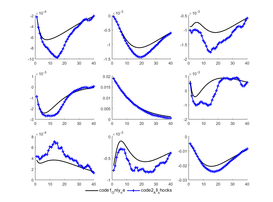
See the figure, the black line the one using the following shocks coding, listing only 1 shock out; the blue line is the results using the shocks coding, listing all shocks out; while all other parts of the mods all the same. The figure that I plotted out using only the es_ne shock, the plotting code is also below.
I believe that these two shocks coding should lead to the same irfs figures, but it turns out to be not!!!See the figure.
I check these twice, there is indeed no difference between these two files, merely the difference at the shocks. I think that even the second one listing all shocks out but I only use the es_ne shock’s result to plot, so it should not bring any difference. But the results shows the difference between these two ways of shocks coding. I never encountered this in the past when solving for 1-order linear models.
Can anyone tell me why? I really want to know the reasons and want to fix it!
%code1_listing_only1shocks
steady; %(solve_algo=1)
check;
shocks;
var es_ne; stderr 0.0199;
end;
stoch_simul(order=2,irf=40,nograph)y c k inv w rk n r mc pi i re rl loan lev_f nw_f lev_m Welf spread;
%code2_listing_allshocks
    steady; %(solve_algo=1)
    check;
    shocks;
    var es_a; stderr  0.0152;
    var es_g; stderr  0.0438;
    var es_v; stderr 0.0130;
    var es_i; stderr 0.0875;
    var es_c; stderr 0.0258;
    var es_ne; stderr 0.0199;
    end;
    stoch_simul(order=2,irf=40,nograph)y c k inv w rk n r mc pi i re rl loan lev_f nw_f lev_m Welf spread;
%plotting matlab code
ending_cell={‘_es_ne’}; %改为技术冲击:ending_cell={‘_e_a’};
HOR=1:1:40;
var={‘y’,‘k’,‘loan’,‘inv’,‘lev_f’,‘rk’,‘pi’, ‘lev_m’,‘Welf’};