Hello,
I’m working with a search-and-matching model that includes output production using capital. My goal is to understand the transition dynamics between two steady states after a labor force shock, using Dynare’s perfect foresight solver.
I’m having trouble with the timing of investment and determining exactly when the shock takes effect. Specifically, I initially defined investment as:
I = K(+1) - (1 - ddd) * K
However, this leads to strange or unexpected results. When I shift the timing and instead define investment as:
I(-1) = K - (1 - ddd) * K(-1)
the behavior of the model becomes more reasonable and aligns better with economic intuition.
Why does this happen? Is it purely a timing convention issue, or is there something deeper about how Dynare handles capital accumulation under perfect foresight?
Additionally, I would like to understand how the perfect foresight solver implements shocks in time :
- If the labor force shock is introduced at time t, does it affect decisions in period t or in t + 1?
- In other words, do agents react in anticipation (since they have perfect foresight), or only after the shock is realized?
I’ve attached the relevant files. Any clarification on Dynare’s treatment of timing in perfect foresight contexts would be greatly appreciated.
Best regards,
Nicolas
solve_SS.m (1.3 KB)
model_dynamic.mod (3.0 KB)
model_dynamic_steadystate.m (1.3 KB)
Thank you very much, Professor Pfeifer. I was able to fix the issue related to capital, but I still have a question regarding the timing of the dynamic response.
In my model, employment and unemployment are defined by the following equations:
U = F - L;
L = (1 - d) * L(-1) + f * U(-1);
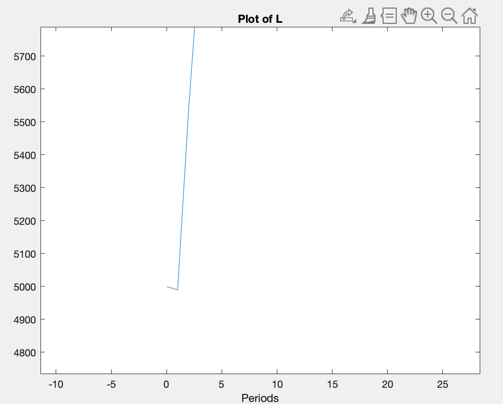
Since the shock occurs at t = 1, I would expect that only unemployment changes in that period, as employment is determined solely by lagged variables (at t-1). However, when I plot the employment response, I notice a slight change in employment at t = 1. Although the change is very small, I expected employment to remain constant between t = 0 and t = 1.
I’ve attached a figure showing the evolution of employment to illustrate what I mean.
Could this be due to numerical precision, or am I misunderstanding the timing?
Thanks in advance!
Which variable exactly are you plotting? And how did you treat the initial condition? If you did not start at a steady state you would expect transition towards the steady state in the first period.
The variable I’m plotting is employment, which I define in the model as L. From what I understand, this variable is determined solely by the equations I mentioned in my previous post. In particular, employment at time t should be fully determined by lagged variables, specifically L(-1) and U(-1), so any change should only be reflected from t+2 onwards.
The simulation starts from the steady state, with an initial condition at t = 0 equal to 5000.13 (the steady state value). However, at t = 1, employment drops to 4989.37. My question is: why does this drop occur at t = 1, if the equations determining employment explicitly depend only on past values.
Thanks in advance!
Without the codes it is impossible to know what is going on.
Sorry, professor. I forgot to attach the files in my last post. Here are the codes.
model_dynamic_steadystate.m (1.3 KB)
model_dynamic.mod (3.0 KB)
solve_SS.m (1.3 KB)
The files do not run, because you load a file that is only created by solve_SS.m, but running that function already requires stst_guess.mat
Sorry again, here is the missing file:
stst_guess.mat (1.6 KB)
In
L = (1 - d) * L(-1) + f * U(-1);
the f is a variable that changes in period 1. That explains why L moves.
Thank you very much, Professor Pfeifer, that was indeed the problem I had.