Time series simulation (simult_) for counterfactual analysis with adaptive learning

Luna · September 16, 2021, 8:56am

What I want to do:
For my master thesis I am estimating the model by Slobodyan&Wouters (2012) with an extended time series. I try to include a counterfactual analysis that investigates what would have happened without the use of unconventional monetary policy. To this end I use the aproach by Mouabbi&Sahuc (2016).

What is the problem?
Before I start with the counterfactual analysis I simulate the time series with the original smoothed shocks from the estimation. In case of the rational expectations version I get back the observed time series as expected. In case of adaptive learning(AL) the simulated time series does not match the data.

Could anyone tell me why this is the case?
My hypotheses are:

I have some kind of error in my code. Slobodyan&Wouters adapted some dynare files - maybe I overlooked a difference in the code that makes it incompatible with “simult_”? (I also manually coded up the simulation as a comparison but I get the same results as simult_.) Any ideas how to proceed in checking if everything is coded correctly?
Under AL this exercise does not necessarily replicate the observed time series. I am using AR(2) learning. In that case I am not sure how to interpret the simulated time series I obtain. Can the exercise still make sense, and should just not be compared directly to observed time series? Or does the exercise make no sense conceptually under AL? (Of course this would be the worst outcome for me.)
In this thread @jpfeifer writes:

What I did so far:
(note that I have to use Dynare 3.6.4 in order to use the toolbox provided by Slobodyan&Wouters (2012))

%Simulation of time series under AL with original shocks:
dynare AL_counterfact_simulation noclearall;
load('AL_extension_4_results.mat', 'dr_') 
load('AL_extension_4_results.mat', 'oo_') 

y0=dr_.ys;
dr= dr_;
iorder=1;
ex_=[oo_.SmoothedShocks.ea oo_.SmoothedShocks.eb oo_.SmoothedShocks.eg oo_.SmoothedShocks.em oo_.SmoothedShocks.epinf oo_.SmoothedShocks.eqs oo_.SmoothedShocks.ew];
y_=simult_(y0,dr,ex_,iorder);

%look at time series (here gdp)
load usmodel_extended_zlb

figure;
plot(dy(71:end), "k"); hold on %data contains training period, start from 71 to start in 1966
%plot(oo_.SmoothedVariables.dy,'r'); hold on
plot(y_(8,:),'b--') %gdp is inrow 8
%plot(oo_.FilteredVariables.dy,'b--');

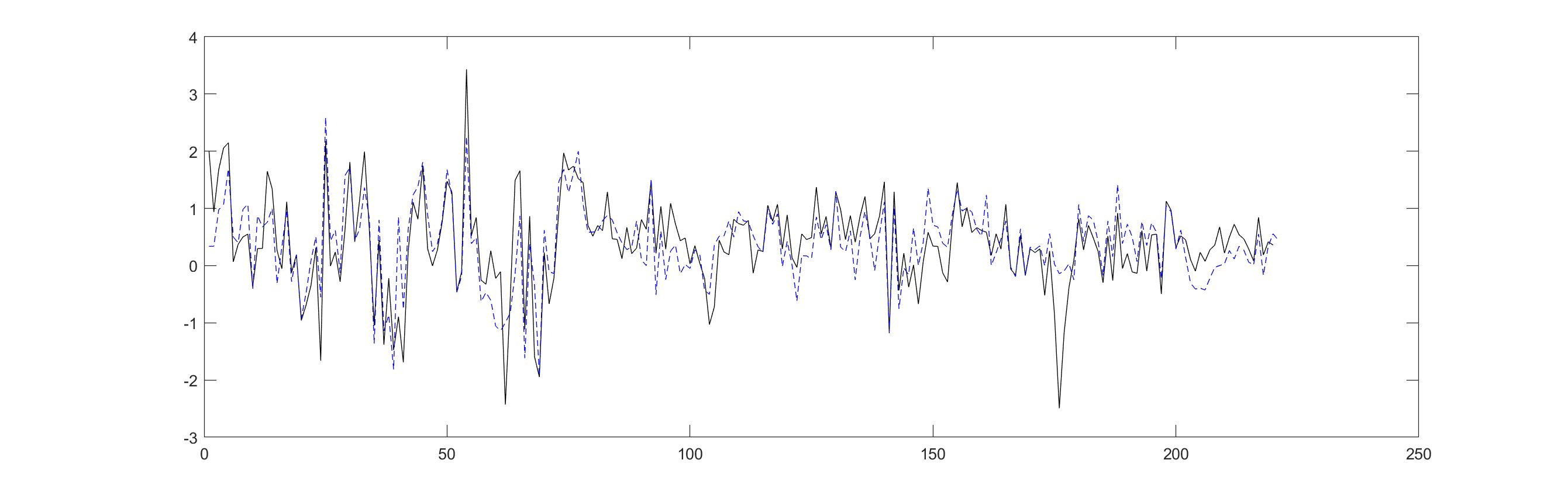
Result under AL (the blue dashed line is the simulated GDP, the black line shows the observed time series):

In case of RE the time series match (I cannot include a second picture as a new user).

The corresponding files are here:
AL_simulation_file.zip (2.6 MB)
RE_simulation_file.zip (773.6 KB)
each folder contains a file called “simulation_file.m” that runs the simulation and loads necessary data.

TL;DR: Simulating time series with original smoothed shocks does not yield observed time series under adaptive learning. Looking for fix or explanation.

Any help would be greatly appreciated!

Thank you

Luna · September 16, 2021, 8:57am

Here is the result for the simulation of gdp under rational expectations:

jpfeifer · September 16, 2021, 9:43am

I am not too familiar with the learning literature. But doesn’t adaptive learning usually imply a time lag between observing variables and reacting them? Depending on the exact timing structure, simult_ may not be appropriate. Maybe an expert like @verdi_green can help.

Luna · September 16, 2021, 1:32pm

Yes, I believe that’s the case. Thank you for tagging @verdi_green, I would really appreciate his help
Just two quick follow up questions:

If a time lag was the issue, could that be sorted by changing the lag structure in the recursive matrix multiplication used to simulate the data, or would that be a deeper rooted problem?
When you wrote this:

did you mean to imply that in case of limited information techniques we would not expect to retrieve the observed data exactly?

verdi_green · September 16, 2021, 8:32pm

Adaptive learning is, basically, computing time-varying transmission mechanism (instead of y_t = \mu + Ty_{t-1} + R\eps_t, one now has y_t = \mu_t + T_ty_{t-1} + R_t\eps_t). Therefore, in order to replicate the results from AL, one needs to save those time-varying objects, and then use them, oo_.SmoothedShocks, and the initial oo_.SmoothedVariables, iterating everything forward.

simult_, of course, will not work, because it simply takes the RE transmission mechanism that’s obtained at the posterior mode and rolls it forward.

Check if the results file has oo_.TT, oo_.RR., and oo_.mus objects. If not, you’ll need to save them yourself in missing_DiffuseKalmanSmoother*.m in or DiffuseKalmanSmootherL1_options_const.m, if you are using DYNARE 4.2.5 (DYNARE 3.61) version.

Luna · September 17, 2021, 9:34am

Ahh yes that makes sense! Thank you for taking the time.

For any future readers, it works for me with this code snippet:

load('AL_extension_16_results.mat', 'oo_') %load result files here
load('AL_extension_16_results.mat', 'dr_')
T = width(oo_.mus)-1;
ex_=[oo_.SmoothedShocks.ea oo_.SmoothedShocks.eb oo_.SmoothedShocks.eg... %provide shocks in alphabetical order here
    oo_.SmoothedShocks.em oo_.SmoothedShocks.epinf...
    oo_.SmoothedShocks.eqs oo_.SmoothedShocks.ew];
y_(dr_.order_var,1) = oo_.mus(:,1);
for i=1:T
    mu= oo_.mus(:,i);
    T = oo_.TT(:,:,i);
    R = oo_.RR(:,:,i);
    y_(dr_.order_var, i+1) = mu + T*y_(dr_.order_var, i)+ R*ex_(i,:)';
end

verdi_green · September 18, 2021, 1:04pm

A correction: you need to start from oo_.SmoothedVariables.pinf(1) for inflation, oo_.SmoothedVariables.y(1) for output, etc. You code starts from the steady state, which means that especially in the beginning the replicated vector y_ won’t be the same as oo_.SmoothedVariables.

Luna · October 1, 2021, 8:45pm

Sorry to bother you again @verdi_green and thank you for pointing out the wrong initialisation! Unfortunately, another issue with the counterfactual analysis has come up:

When simulating the time series for a counterfactual scenario without unconventional monetary policy I exchange the smoothed shocks series for the monetary policy shock and keep all other shock series constant.

What I did so far:

exchange \epsilon_t[4] (the MP shock is in the 4th row)
exchange R_t[,4] (insert the 4th column from the counterfactual estimation that I performed to obtain the alternative shocks)
simulate the alternative time series with y_t = \mu_t + T_ty_{t-1} + R_t\epsilon_t

The issue:
Obviously, y_{t-1} are different from period 2 on but I still used the original T_t. If I am not mistaken this only takes into account the “direct effect” on the transmission of different monetary policy not the indirect effect through changed transmission of all the model’s variables.

My question:
Is there a way to recover the T_t that is in line with y_{t-1} obtained with the counterfactual R_t\epsilon_t?

I hope the question makes sense. Any input would be greatly appreciated.

verdi_green · October 2, 2021, 11:09am

Luna,

Basically, if I understand correctly what you want, you need to take the entire estimation code, and replace the data vector Y in line

v = Y(:,t) - a(mf);

with the counterfactual y_t that you generated, based on SmoothedShocks with your added or removed MP shocks. The new counterfactuals serve only to produce the measurement error, and then the Kalman filter proceeds as usual, the agents update beliefs, construct new T and R, etc. In the end, you will get a new sequence of TT, RR, and mus, new beliefs, and new counterfactual “data”.

Luna · October 5, 2021, 4:09pm

Thank you for the explanation! And please excuse the delayed reply - I was sick the last couple of days.

When I follow the steps as I understand them I retrieve again the counterfactual y_t from above. Maybe I missunderstood some step.

I replaced Y with my counterfactual y_t in both “DiffuseKalmanSmootherKMAL1_options_const.m” (line 198) and “DiffuseLikelihoodKMAL1_options_const.m” (line 191)
(I used Kalman filter learning with a constant)
With this change I ran another estimation (I did not re-estimate the parameters) which leads to a “new” sequence of TT,RR, mus,…
When I take the newly calculated TT, RR and mus matrices as well as my counterfactual set of shocks and simulate the model, I get counterfactual “data” that is almost identical to the y_t from above.