Strange IRFs + problem with consumption

Bohdan · February 12, 2025, 7:55am

Dear Dynar community,

I am trying to replicate the paper of Gawthorpe, K. (2019). which in turn is based on Aliyev, I., Bobková, B., & Štork, Z. (2014) on the NK SOE model of the Czech economy.

The model presented in the papers incorporates price and wage rigidities, has a fiscal policy with taxes, and government consumption and can run a budget deficit, and has a monetary policy with the Taylor rule as well as other features.

The model in the paper is log-linearised, but I would like to replicate the nonlinear model instead.
In addition, I am adding material inputs to the intermediate producer’s Cobb-Douglas production function, as I want to achieve the input-output sectoral model from the paper of Gawthorpe.

I am new to DSGE, therefore I am approaching the replication of the paper step-by-step by gradually increasing the complexity of the model.
In this phase, I have the model for a closed economy, but with fiscal policy and monetary policy.

I have faced two main problems with it so far:

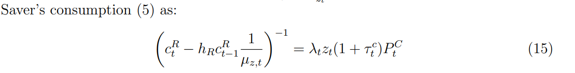
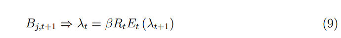
First, the model does not allow for the Euler equation of consumption to be solely determined by monetary policy rate. I studied the reason behind it and found that it requires consumption to be defined by the return on capital - otherwise, it does not reach a steady state. Incorporation of the relation of the monetary policy rate with return on capital such as \frac{R}{\Pi_{t+1}} + \text{Risk} = \frac{R_K (1 - \tau_K)}{P_K}, where R is a monetary policy rate defined by Taylor rule, Pi is inflation, R_K is a rate on capital and P_K is a price of capital and tau_k is a tax on capital did not help - due to conflict with monetary policy rule and rate on a capital equation.
In order to deal with it I employed a temporary solution - consumption depends on a rate of capital and monetary policy rate with equal weights of 0.5, but this does not solve the core problem.
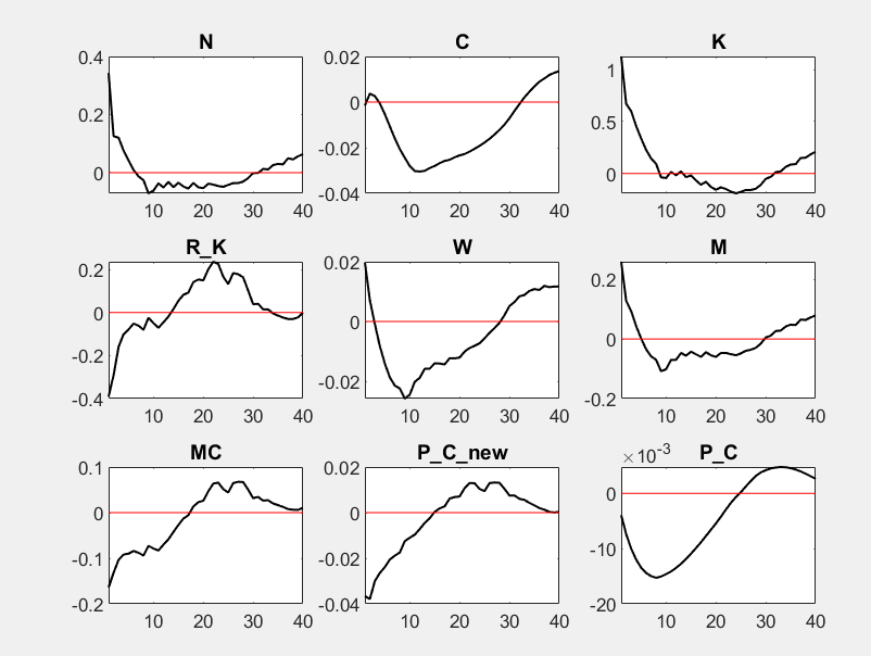
The model produces very strange IRFs:

image802×604 16.2 KB

In addition, if I change a fraction of firms that do not re-set
their prices in respective period ( ζ ) to a lower value, the model violates Blanchard & Kahn conditions. If I change the elasticity of substitution between different goods (θ) to any other value apart from 2, the model does not reach the steady state.
I studied the potential problem behind it and my hypothesis is that it is due to the addition of forward-looking expectations for the new price, which is set by:

\Xi_n = P_C^\theta Y_F MC + \zeta \beta \Xi_n^{(+1)};

\Xi_d = P_C^{\theta - 1} Y_F + \zeta \beta \Xi_d^{(+1)};

P_C^{\text{new}} = \frac{\theta}{\theta - 1} \frac{\Xi_n}{\Xi_d} + \epsilon_{P_C};

, where MC is marginal costs and Y_F is a final production.
When I tried the simpler model, in which the new price is determined only by a mark-up and future marginal costs

P_C^{\text{new}} = \frac{\theta_w}{\theta_w - 1} MC^{(+1)}

, the model seemed to work fine (at least IRFs were appropriate).

Any help or suggestions on how to deal with these problems would be much appreciated!

Paper of Gawthorpe, K. (2019)
Czechia.pdf (1009.4 KB)

Paper of Aliyev, I., Bobková, B., & Štork, Z. (2014)
Extended-DSGE-Model-of-the-CZ-economy (1).pdf (588.4 KB)

My current model
Autarky_last.mod (3.5 KB)

Thank you in advance.

jpfeifer · February 12, 2025, 7:59pm

There are almost surely timing errors. K_S should be predetermined.
You should set order=1. With order=2, you need a lot more repetitions to get smooth IRFs.

Bohdan · February 13, 2025, 1:27pm

Dear Prof. Pfeifer,

Thank you a lot for the feedback. In the case of 2, your solution worked perfectly, IRFs are far smoother.

In the case with 1, the model does not reach a steady state if I specify

\frac{C^{(+1)} - h C}{C - h C^{(-1)}} \times \Pi^{(+1)} \times \left( \frac{1 + \tau_C^{(+1)}}{1 + \tau_C} \right) = \beta R

instead of the equation I currently have in the model (which makes consumption dependent not only on R - monetary policy rate but also on R_K - return on capital) and define K_S (capital stock) as predetermined. I also tried to define K (capital) or U_K (utilisation of capital) as predetermined, but unfortunately, it also did not help.

The inclusion of the Risk variable and R_K/R relation with the formula

\frac{R}{\Pi_{t+1}} + \text{Risk} = \frac{R_K (1 - \tau_K)}{P_K}

also does not seem to assist the model to reach the steady state.

jpfeifer · February 14, 2025, 10:14am

What you describe suggests a problem in your equations/calibration. It sounds as if the two Euler equations for bonds and capital are inconsistent.

Bohdan · February 14, 2025, 12:04pm

Excuse me, maybe I explained it unclearly - I meant that there should be only one Equler equation for consumption, which would be dependent only on the monetary policy rate and not on the rate of capital.

But if I specify it in the code to be dependent only on the monetary policy rate (and if I do not employ the rate on capital), the model does not reach the steady state.

jpfeifer · February 14, 2025, 12:16pm

The first equation clearly shows that in steady state it needs to hold that

R/\Pi=1/\beta

Does that hold in your model?

Bohdan · February 14, 2025, 12:47pm

Prof. Pfeifer,

It seems that yes. In the source paper, the Euler equation for consumption is derived from:

and

beta * R is placed on the RHS of the consumption equation by substituting lambda/lambda(+1) with beta * R.

The log-lin version looks like this:

I checked the derivations and calculus, it should be correct

jpfeifer · February 14, 2025, 2:14pm

Then you need to find out what is wrong in your implementation, which gives you an incorrect steady state.

Bohdan · February 14, 2025, 2:32pm

Thank you! Might it be in consumption Euler, or maybe somewhere else in other equations?
I tried to find the source of the problem and the only thing I defined (by steadily simplifying the model) is that the model needs consumption to be defined by the return on capital in some form, else it doe not reach a steady state.

Bohdan · February 15, 2025, 1:00pm

Just in case anyone needs the current code, it is here a bit down.

THe problem is with consumption Euler, RHS should be “= beta*R”, but in this case the model does not reach the steady state:

var N C K R_K W M MC P_C_new P_C P_M P_K P_I B Q Y_I Y_D I Pi R  A K_S U_K TQ GR GC GE Xi_n Xi_d Y_F; 

varexo eps_Y eps_A eps_Pc eps_W eps_GC eps_R ;

parameters h psi delt k alph gamm zeta theta beta phi lambda_Pi lambda_Y tau_C tau_K tau_W R_bar;

beta = 0.99; 
h = 0.8;       //consumption habits
psi = 1.55;    //inverse of substitution of labour supply
delt = 0.04;   //ammortisation of capital
k = 11;        //parameter of investment adjustment costs function
alph = 0.33;   //share of capital in productiona
gamm = 0.17;   //share of material inputs in producation
theta = 2;     //elasticity of substitution between different goods
zeta = 0.9;    //fraction of firms that do not re-settheir prices in respective period
phi = 0.25;    //lag of monetary policy
lambda_Pi = 1.5;  //inflation weight in MP rule
lambda_Y = 0.25;  //output weight in MP rule
tau_K = 0.18;    //tax on capital
tau_C = 0.2;     //tax on consumption
tau_W = 0.215;   //tax on wages
R_bar = 1/beta;  //Steady-state interest rate


model;

//Inflation
Pi = P_C/P_C(-1);

//Technology
A = 0.5*1 + 0.5*A(-1) + eps_A;

//Utilisation rate of capital
U_K = 0.5*R_K*(1-tau_K)/P_K;

//Labour supply
N^psi =  W*(1-tau_W) /( P_C*(C - h * C(-1) ) * (1 + tau_C) );
 
//Consumption Euler
( C(+1) - h*C ) / ( C - h*C(-1) ) * Pi(+1)* ( (1+tau_C(+1))/(1+tau_C) ) =  0.5*1/TQ * ( beta*(1-delt)*TQ(+1) + beta*R_K(+1)*U_K(+1)*(1-tau_K(+1)) - P_K*( 2*(U_K(+1) - 1) +  (U_K(+1) - 1)^2 ) ) + 0.5*beta*R; 
//( C(+1) - h*C ) / ( C - h*C(-1) ) * Pi(+1)* ( (1+tau_C(+1))/(1+tau_C) ) =  beta*R;

//Capital stock accumulation
K_S(+1) =   K_S*(1 - delt) + I*(1 - k/2*(  I/I(-1) - 1  )^2);

//Capital and capital stock relation
K = K_S*U_K;

//Tobin's Q
TQ*R =  (1-delt)*TQ(+1) + (1-tau_K(+1))*R_K(+1)*U_K(+1) - P_K(+1)*( 2*(U_K(+1) - 1) +  (U_K(+1) - 1)^2 ); 

//Return on capital
R_K = alph*Y_I*MC/K;

//Wages
W = Y_I*MC/N*(1 - alph - gamm) + eps_W; 

//Material imput
M = gamm*Y_I*MC/P_M;

//Marginal costs for intermediate producers
MC = (R_K^alph)*((1/alph)^alph) * (P_M^gamm)*((1/gamm)^gamm) * (W^(1 - alph - gamm))* ((1/(1 - alph - gamm))^(1 - alph - gamm) );

//Nominator and denominator for the new price
Xi_n = P_C^theta * Y_F * MC + zeta*beta*Xi_n(+1);
Xi_d = P_C^(theta - 1) * Y_F + zeta*beta*Xi_d(+1);

//New price
P_C_new = theta/(theta - 1)*Xi_n/Xi_d + eps_Pc; 

//Current prices, dependent on a lag of prices and a new price
P_C = ( zeta*P_C(-1)^(1 - theta) + (1 - zeta)*P_C_new^(1 - theta) )^(1/(1-theta) );

//Prices on material input, capital and investments
P_M = P_C;   
P_I = P_C;   
P_K = P_C;


//Final producers production
Y_I = Y_F*(P_C_new/P_C)^(-theta);

//Intermediate producer's production
Y_I = A*(K^alph)*(M^gamm)*(N^(1 - alph - gamm));

//Revenue of intermediate producers
Q = Y_F*P_C - W*N - R_K*K - P_M*M ;   

//Gov revenue
GR = tau_C*(P_C*C + GE*P_C) + tau_W*(W*N) + tau_K*(R_K*K + Q);

//Gov consumption
GC = 0.4*GC(-1) + 0.6*0.1 + eps_GC;

//Gov expenditures
GE = GC;                           

//Gov debt   
//GE - GR = B - B(-1)*R;
GE - GR = 1/R*B(+1) - B;

//Aggregate demand                                                      
Y_D = I + C + GE/P_C + eps_Y;

//Equlity of aggregate demand and aggregate supply
Y_F = Y_D;

//Monetary policy
R = (1-phi)*(R_bar + lambda_Pi*( P_C/P_C(-1) - 1 ) + lambda_Y*( Y_F/Y_F(-1) -1 )) + phi*R(-1) + eps_R; 



end;

predetermined_variables K_S;


initval;
B = 0;


end;

steady(maxit=1000,solve_algo=4);
model_diagnostics;


check;


shocks;

var eps_R; stderr 0.03;


end;


stoch_simul(order=1, pruning);

jpfeifer · February 15, 2025, 1:48pm

You need to provide initial values for all endogenous variables. And you still did not address the unit root problem in the price level.

Bohdan · February 15, 2025, 5:03pm

Prof. Pfeifer,

Thank you for the feedback again. I will come up with steady-state model part, I have thought about that earlier, but so far the model worked without it.

I am not sure I understand why the unit root problem in the price level is present now - IRFs are a bit strange, but they do not seem to show a unit root behaviour

jpfeifer · February 16, 2025, 11:56am

As mentioned above, in New Keynesian models only the inflation rate is uniquely determined, not the price level itself. Most models have a zero inflation steady state. But any initial price level, e.g. P=1 or P=10000 would be consistent with that.

Bohdan · February 17, 2025, 10:47am

Prof. Pfeifer,

Than you a lot for your feedback. I will try to implement the changes you have mentioned.

Bohdan · March 10, 2025, 12:42pm

Prof. Pfeifer,

Could you please give me a hint on how to address the unit root problem in the price level?
I assume I have to divide some of the nominal variables, such as GDP and wages by the price level, but I am not sure if I am right.

jpfeifer · March 10, 2025, 5:52pm

Typically, you can express the model in real quantities and inflation rates. The nominal wage should not show up, only the real wage. You can define W_real=W/P.

Bohdan · March 11, 2025, 12:06pm

Thank you!