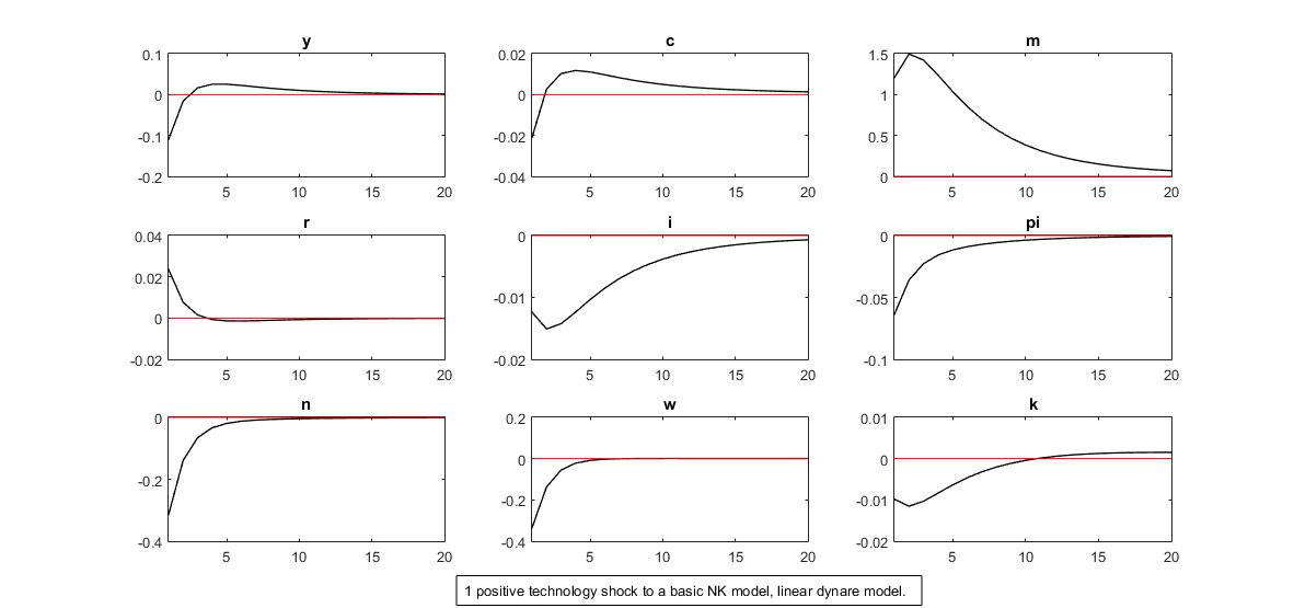
I have a question about the differences on impulse response pictures of linear dynare model and non-linear. When I run a basic NK model (I use a log-linear model in dynare)and add a positive productivity to see the result. Output changes from negative to positive and then goes back to steady state. And, my question is, how can output be negative at period 0? It is a positive technology shock! Even though the impulse response picture of output is hump shape, I still don’t know how to interpret this result.
Please help!
Many Thanks in advance!
In relation to this thread, if we have a multi-sector model, for example, with an export sector (yxt), a non-tradable sector(ynt), a domestic tradable sector(ydt) and a foreign tradable sector(yft), can aggregate output (y) then be negative in the first period even if a positive productivity shock in the non-tradable sector increases and hence ynt increases? For example, because output in other sectors may be negative at period 0.
Hello, you could also share your mod file, maybe someone can have a look. A simple question, did you check and confirm that the irf of the shock variable shows a raise as you intend?
Hi Fernando, yes, the shock variable itself shows a raise. I am having this problem with productivity shock in the domestic tradable sector. Domestic tradable output increases as expected but aggregate output (which involves all sectors) falls. The model is kinda large (about 90 equations), I will start building again, hopefully I may spot the mistake. Otherwise, I will share my mod file here. Thanks!
Ok, I see, as you say, perhaps trying to build up the model again can help. When I have replicated models with different, let’s say, “n” productive sectors, sometimes I tried a generalized productive shock affecting all the “n” production functions, then I shock again in “n-1”, “n-2” and so on production functions. Perhaps that can give you an idea of what’s happening in your model when the shock affects only in the tradable sector.
If you don’t mind, may I ask how you normally extend your closed economy model to an open economy model, particularly regarding the introduction of foreign bonds, foreign interest rates and exchange rate into the model?
With the introduction of these 3 new variables into the model, I kind off need 3 new equations for dynare to run the mod file.
Sometimes, I add a UIP equation (i.e., combining Euler equation for domestic and foreign bonds), an AR(1) process for foreign interest rates and an AR(1) process for the exchange rate. But obviously they become collinear although the model is sometimes able to run. Other times I get collinearity error.
My observation from some papers is that we can assume that domestic bond is 0 in equilibrium, and hence gets dropped from the model while adding the 3 new variables. So technically, we just need to add two new equations - UIP equation and AR(1) process for foreign interest rates. Although research papers don’t build models step by step in this manner (like building a closed economy model first and extending it), I suspect this is one feasible option to avoid collinearity.
Also I have seen that some papers even assume a zero foreign interest rate and hence they just need to introduce Euler equation for foreign bonds and an AR(1) exchange rate shock, together with 2 new variables - foreign bonds and exchange rate. I suspect this is another way to avoid collinearity. Not sure though.
Recently I found out that I can avoid the collinearity problem by introducing a UIP equation, a foreign interest rate shock and a net foreign asset position equation when I extend a closed economy model to incorporate foreign interest rates, foreign bonds and exchange rate. Not sure though if there exist some standard way to do this.
Hello, I am not sure how useful I am on this regard, perhaps @jpfeifer can help on it.
If you are investigating the responses after a shock in the exchange rate, then to use it as an AR(1) seems correct to me, hence you can do what you say in here:
But as you say, you will face colinearity and the domestic rate moves along in the same proportion. This happens unless you have a portfolio adjustment cost of acquiring more/less foreign bonds, hence the UIP changes, see Eq5 in Chang, C., Liu, Z., & Spiegel, M. M. (2015). “Capital controls and optimal Chinese monetary policy”.
I am not pretty sure about this option:
In general terms, if I am not mistaking, adding foreign bonds, exchange rate and foreign interest rate in a SOE require the foreign rate equation (an AR(1) is an option), the FOC with respect to foreign bonds, and the UIP or balance trade/current account equation that balances home to foreign goods/bonds.
Given that a small open economy implies that it does not affect the foreign economy, you can indeed select the foreign interest rate as you like. It can be an AR(1). But you can also assume that it is just a number.
Talking about collinearity is not helpful, because it can be due to a unit root (which is common in SMOPEC models due to non-stationarity of the net foreign asset position), which is not a problem, or entering redundant information and therefore missing crucial information to pin down the endogenous variables.
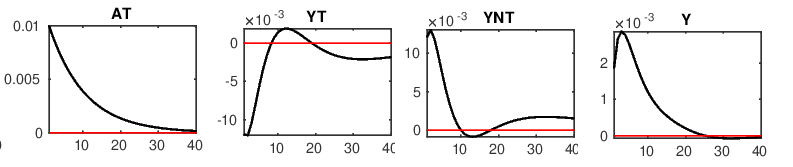
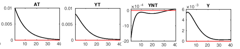
I have tried to debug my model by building it again. I have figure out the stage where the productivity shock (eT) in the tradable sector reduces tradable sector output (YT) instead of increasing it. Aggregate output (Y), however, increases though.
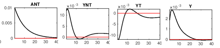
Productivity shock (eNT) in the non-tradable sector is ok as both non-tradable sector ouput (YNT) and aggregate output (Y) increases. IRFs seems to be the same though, as in the tradable sector.
Other results seem ok too. But I have realized that IRFs related to the tradable sector are the exact oposite of IRFs in the non-tradable sector. And this is perhaps causing tradable sector ouput (YT) to negatively respond to tradable sector productivity shock (eT).
Unfortunately, I have not been able to see where the problem is coming from. Thus, which equation may be causing this. Maybe, you may have encountered such a problem before.
I have attached the baseline model with one production sector (baseline.mod (8.1 KB) ), and the extension (extension.mod (9.5 KB) ) with tradable and non-tradable sectors.
But lemme write them here for an easy check. So basically, I drop these equations from the baseline model:
//FIRMS//
//14-Production Function
Y = A + alpha1*(U+KP(-1)) + alpha2*L + alpha3*KG(-1);
//15- Problem of the firm trade-off (MRS=Relative price)
L - U - KP(-1) = R - W;
//16-Marginal Cost
CM = alpha2*W + alpha1*R - A - alpha3*KG(-1);
//17-Phillips Equation
PI = beta*PI(+1) + ((1-theta)*(1-beta*theta)/theta)*(CM-P);
//18-Gross Inflation Rate
PI(+1) = P(+1) - P;

And I replace them with the following equations in the extended model:


    YNT = ANT + alpha1*(U + KNT) + alpha2*LNT + alpha3*KGNT;
    //FOC of non-tradable firms - MRS
    LNT - U - KNT = R - W;
    // Marginal cost
    MCNT = alpha2*W + alpha1*R - ANT - alpha3*KGNT;
    //Phillips equation
    PINT = beta*PINT(+1) + ((1-theta)*(1-beta*theta)/theta)*(MCNT-PNT);
    //Non-tradable sector inflation
    PINT(+1) = PNT(+1) - PNT;

    //DEMAND FUNCTIONS IN THE NON-TRADABLE SECTOR
    CNT = zeta1*(P-PNT) + C;
    INTT = zeta1*(P-PNT) + IP;
    IGNT = zeta1*(P-PNT) + IG;
    GNT = zeta1*(P-PNT) + G;

    //MARKET CLEARING IN NON-TRADABLE GOODS SECTOR
    YNTss*YNT = CNTss*CNT + INTss*INTT + IGNTss*IGNT + GNTss*GNT;

    // TRADABLE SECTOR
    //Production function
    YT = AT + alpha1*(U + KT) + alpha2*LT + alpha3*KGT;
    //FOC of tradable firms - MRS
    //Tradable firm's labor demand
    LT = MCT + YT -W;
    //TRadable firm's capital demand
    KT = MCT + YT - R - U;
    //Marginal cost
    MCT = alpha2*W + alpha1*R - AT - alpha3*KGT;
    //Phillips equation
    PIT = beta*PIT(+1) + ((1-theta2)*(1-beta*theta2)/theta2)*(MCT-PT);
    //Tradable sector inflation 15
    PIT(+1) = PT(+1) - PT;

    //MARKET CLEARING FOR PRIVATE CAPITAL
    KP(-1) = KT + KNT;
    //MARKET CLEARING FOR GOVERNMENT CAPITAL
    KG(-1) = KGT + KGNT;
    //MARKET CLEARING FOR LABOR
    L = LT + LNT;

    //GROSS INFLATION RATE
    PI = omega1*PIT + (1-omega1)*PINT;
    //AGGREGATE PRICE
    P = omega1*PT + (1-omega1)*PNT;

//Aggregate supply
Yss*(Y) = (PNTss/Pss)*YNTss*(PNT + YNT - P) + YTss*(PTss/Pss)*(PT + YT - P);
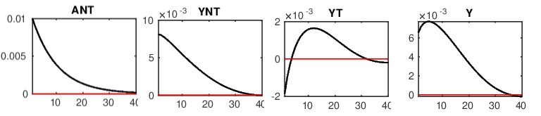
Thanks, Prof. Pfeifer, I rewrote the production sector of the economy again without PINT(+1) = PNT(+1) - PNT and PIT(+1) = PT(+1) - PT…and it works.
Productivity shock in the non-tradable sector appears correct.
But still not clear to me why we should drop equations like these: PI(+1) = P(+1) - P aside causing unit root problems. The last time, I understood that unit roots are not necessarily a problem if the mod file is able to run.
Indeed, in this book:Understanding DSGE models, the author always uses PI(+1) = P(+1) - P and PIW(+1) = W(+1) - W in all their price and wage stickiness models. I actually took my baseline model from there.
I have never seen that book, but from what I see here, it not trustworthy. The problem with the equation is not the unit root, it’s the timing, which means in Dynare: E_t\pi_{t+1}=E_tp_{t+1}-p_t
while the correct definition in Dynare is \pi_{t}=p_{t}-p_{t-1}
i.e. it has to hold always, not just in expectations.
Hello, Emmanuel, sorry I couldn’t reply before. As Johannes points out, try to check the timing in the equations and those definitions. I normally choose either to use price level or inflation in the whole set of equations. Together with inflation definition, the market clearing for both types of capital is not very conventional, well, as far as I know. I am glad your code shows what you were expecting, I would just recheck those timings that I point out.
I see that you follow the book of Celso Costa, so as his MOD example, you could also ask him about these issues on the inflation definitions and the problems that you encountered when trying to replicate. I am sure he can give you insights of his code.
Hi Fernando, thanks for the reply. Indeed, I also got rid of the market clearing for government capital when I removed the incorrect timing for inflation.