Hi everybody,
I am simulating the transition from a steady state with no tax on emissions to a steady state with positive tax in a e-dsge model.
Some trajectories exhibit quite strange behaviour (e.g nominal rate, inflation, asset prices) but I am pretty sure about the timing as the model is quite simple at this stage.
If I use as a sequence of shock a linear increase from 0 to the value declared in the endval; block of the attacched code rather than a fixed tax schedule, or some other smooth sequences, the situation gets even worse.
Does anybody have some insights?
Thank you so much for your assistance
edsge_nobank.mod (7.6 KB)
edsge_nobank_steadystate.m (2.4 KB)
findssedsge_nobank.m (1.7 KB)
What exactly do yo find unusual. Hump shaped overshooting happens quite regularly in such models. But you need more periods (like 2000) for proper convergence to the terminal steady state at the end.
Sorry to re-open the post, but what I find unusual is somehow trickier.
I can’t understand why, when I change the tax schedule to an increasing one and activate the shock block (i.e. a tax schedule that increases in the first 99 quarters, like the one below), the dynamics of the nominal variables become quite strange during the period in which the tax increases. Could it be a matter of terminal points?
I specified the endval point as the last point in my schedule, but the dynamics are still weird.
carbontax.mat (1000 Bytes)
example.m (100 Bytes)
Thank you very much
What do you mean with strange? The IRFs do not look unusual to me. With a long anticipation horizon, there will be a lot of intertemporal substitution going on.
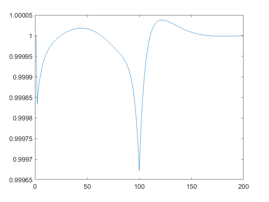
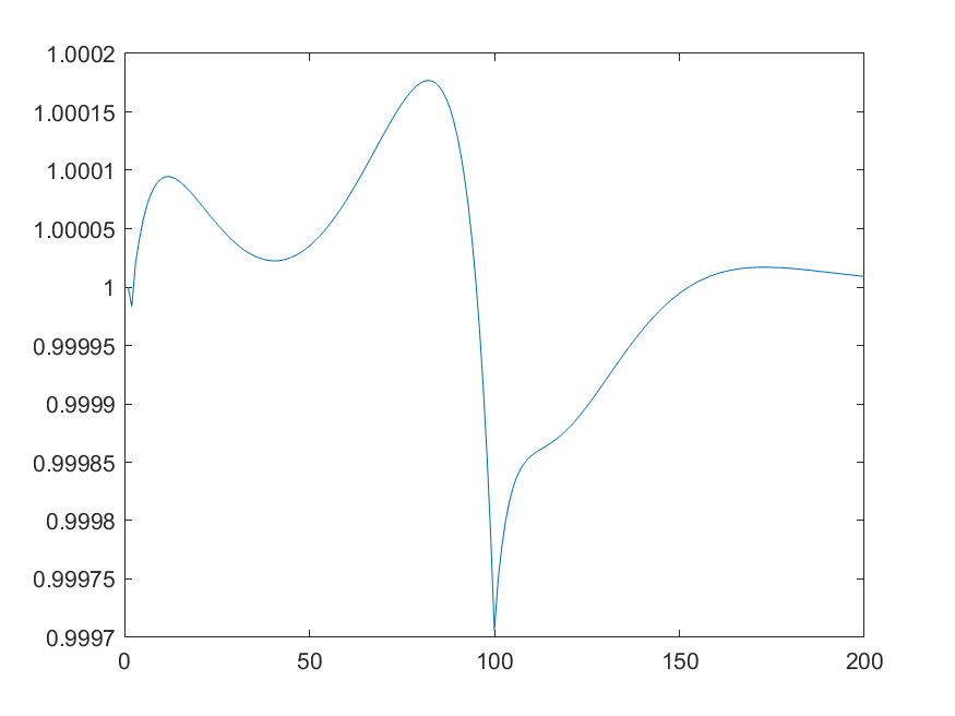
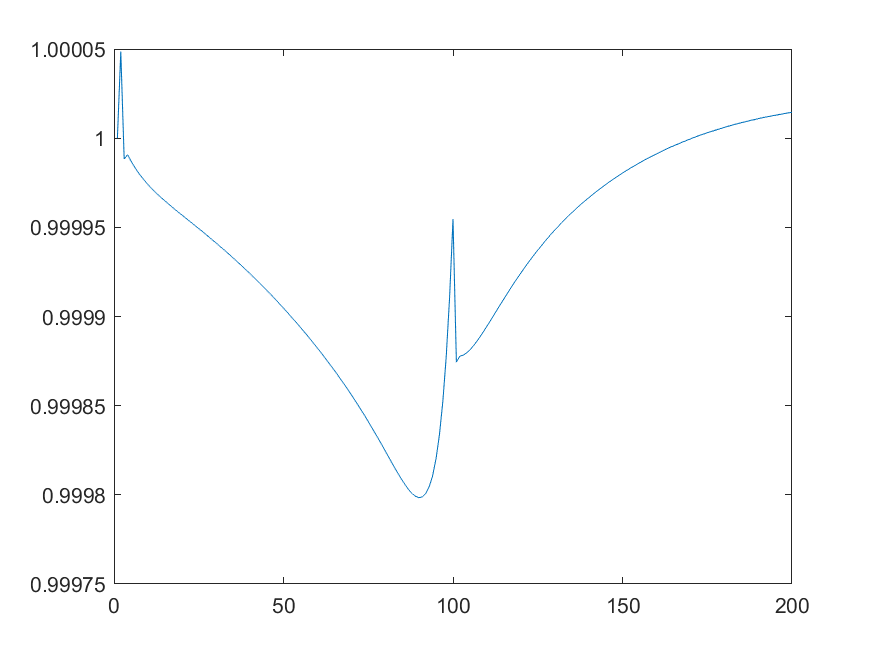
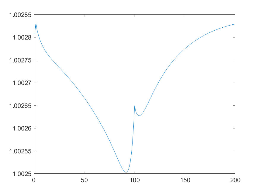
By strange I mean that the shape in the time span in which the tax schedule is increasing (first 100 periods of the 2000-periods simulation) is quite irregular and does not allow for an economic interpretation .
For example, here is the plot of the first 200 periods of the brown and green asset prices, inflation and the nominal rate. However, the same argument would apply even if I only plotted the first 100 periods.
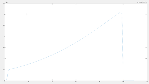
That seems to be due to the not uniformly smooth path for taxes. If you plot the tax changes, you get
The two kinks between period 99 and 101 cause the movements you describe.
this is the growth rate of the tax, correct?
-
Actually if I only care about the transition period (ie. the period in which the tax is increasing, that is, the first 100 quarters), I can cut the time-horizon of the perfect foresight solver to 100 periods only? or it would be a conceptual error as I would not achieve a real convergence since the variable, I guess, would jump abruptly to the new steady state at t=100?
-
Alternatively, is it correct to artificially lenghten the tax schedule to t=2000 (or t=100+(arbitrary number)) so as to avoid the sudden drop of the growth rate you have plotted in the figure, and obtain smoothness in the first 100 quarters (which I only care about)?
Thank you very much for you help
That was the change in taxes, not the growth rate, i.e. abolute differences, not log differences.
No, you cannot simply cut off simulations. Agents are assumed to know the full path of shocks and and will react to these. After the last shock has realized, transition to the new steady state will still take time due to endogenous propagation via stocks like capital.
Again, the last movements do not seem to be a cause for concern. You may want to smooth out the kink between period 99 and 100. The one from 100 to 101, when the tax rate stays constant, is unavoidable.
