I am doing a bit of a policy analysis, in which I need to stochastically simulate a certain periods of observables y, pi, R, based on historical data y, pi, R. Here’s how I plan to do it.
1.1. Fix other parameters, loop over the policy parameters, for each loop:
1.2. Set multiple seeds, draw distribution of p( y_t+s, pi_t+s, R_t+s | y_t, pi_t, R_t) using histval (initval should still be the steady state values,right? Can i change the histval in matlab using some set_ commands as well?), find the expected welfare at this parameter value.
2. Compare the welfare across policy parameters and find the optimum.
However, I have no idea how to generate a distribution of observables with multiple seeds (the 1.2 step). Should i just set_dynare_seed(i) in matlab, and call stoch_simul(M_, options_, oo_, var_list_) after first_time=1? Or maybe I’m doing this in a silly way, there’s in fact a much better way to do this?
What exactly is the interpretation of the exercise you are trying to conduct? You have a bunch of observables but don’t know the value of the state variables? And now you want to take into account uncertainty about what exactly? The initial condition?
Sorry for the confusion, the exercise is to compare welfare loss under different parameter settings (including policy parameters e.g., taylor rule).
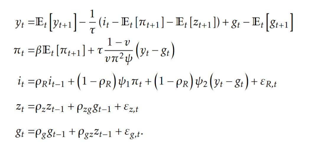
I have a history of observed variables y, pi, R and a model with uncertain range of parameter values. Think of the standard easiest 3-eq NK model.
Now I want to simulate forward y, pi, R based on this history (hence maybe the histval), but using all the possible parameters (maybe a grid search or optimization within a range of values).
For each parameter, the simulation should be a distribution of y, pi, R (randomness comes from the shocks. That’s why I asked about multiple seeds, cause I was thinking multiple stoch_simul), then I average over these results, find the expectation for the welfare under this parameter setting, and compare welfare for each parameter.
I am still confused. The 3 equation New Keynesian model is a linearized model without any states. In that case, the history is irrelevant and you could go for theoretical welfare objects instead if simulated ones. This only changes if you go to second order (which is generally required for welfare comparisons). But then what matters is the value of the state variables (in case of conditional welfare), not the value of the observables. But the value of these state variables will be a function of past shocks on the parameter values. I don’t see how you can only consider parameter uncertainty and completely abstract from state uncertainty (unless there are no states or you are making implicit assumptions).
Thanks for your reply. Let me be more specific with the model. The model above is AS2007, z, g, R are the states, y pi R are observables. And yes I have all the variable history including z, g, R, y, pi (sorry for mentioning only the observables). I am dealing with the linearized NK. Welfare loss is in the form E_{t=0} \sum \beta^s [ a\cdot y_{t+s}^2 +b \cdot\pi_{t+s}^2 ].
I believe the trajectory of y(0), pi(0), R(0) and forward depend on past z(-1), g(-1), R(-1)? And all I need is to simulate the shocks? Are you saying I should directly compute the welfare loss based on policy function coefficients?
Here’s the new plan:
For each parameter, solve for the state space form (z_t,g_t,R_t,y_t,\pi_t) '= A\cdot (z_{t-1},g_{t-1},R_{t-1},y_{t-1},\pi_{t-1}) '+B\cdot (e_{t}^z,e_{t}^g,e_{t}^R)'. E_{t=0}(y_{t+s}^2+\pi_{t+s}^2)= \left[A(4,:)\cdot A(1:3,:)^{s-1}\cdot (z_{t=0},g_{t=0},R_{t=0})'\right]^2+ \left[A(5,:)\cdot A(1:3,:)^{s-1}\cdot (z_{t=0},g_{t=0},R_{t=0})'\right]^2 + \text{ some term that consists of } \sigma_z, \sigma_R, \sigma_g
No need to simulate anything, just solve and compute. Sounds reasonable?
I see, so your model indeed features endogenous states and you are interest in conditional welfare.
The issue is you don’t know the initial condition for e.g. r_0 at the beginning of the sample. That’s why you can’t do the computation you outlined unless you condition on the initial values being e.g. at the steady state (essentially a conditional likelihood).
Thank you! In fact I have simulated z,g,R,y,\pi from t= -200 to t=0, so I can and I did that computation conditional on z_0,g_0 and R_0 mentioned here (Stoch_simul with multiple seedss - #6 by Kylekk) yesterday.
What I found really annoying is the welfare related optimal policy parameters are very sensitive to the initial states z_0,g_0 and R_0 (optimal Taylor rule parameters \psi_1 and \psi_2 vary a lot with a different initial state and this magnitude of \psi does not seem about right, when I do not set a upper bound for them).
Do you have an idea of what might go wrong? Even when I let z,g,R=0 for the t=0, the optimum for them is around \psi_1=70 and \psi_2=30 when what I really want to see is around 1.5 and 1. I guess my question is, what is the force that could be used to drag these two numbers down that i’m missing? compute_loss.m (1.3 KB)
Conditional welfare will of course very much depend on the initial state. If TFP z_= is really high, agents naturally a lot better off. That’s why fair comparisons keep the condition fixed.
Depending on the nature of shocks, it is very common that optimal rules involve full stabilization of inflation (infinite weight on inflation). In the basic NK model, divine coincidence holds. The central bank should completely stabilize inflation.
I see, I completely forget about this… When the shocks move output and inflation in the same direction and they both depend on nominal rate with same sign. Stabilizing one is stabilizing another. Is there a minimum twist of this model (without adding too much feature) that makes policy analysis nontrivial?
Because I am trying to showcase an example where parameter uncertainty could lead to policy uncertainty.
My work is on how to identify the range of parameters (when the model is not identified). And to show this is important in policy-making, I would love to have an easy example (in this case AS2007, which is famous for non-identification in certain parameters) in which different parameters would lead to different policies.
Sorry, I might not get what do you mean by ‘strength’. My understanding is the existence of a trade-off depends on two things: 1. Whether or not output gap and inflation move in the same directions in response to a shock. 2. whether the policy decreases output gap also decreases inflation.
Are you saying i should try different calibration of coefficients in front of those shocks?
Yes, but demand shocks move the ouput gap and inflation in the same direction, while supply shocks move them in opposite directions. Thus, the optimal response to each of these shocks in isolation is different. For a realistic mixture of shocks, the optimal coefficients should be more normal.