Dear Prof. Pfeiffer,
I am currently developing a small open economy (SOE) environmental model following Gali’s textbook, formulated in its non-linear form. My model includes two sectors (green and brown) and domestic importers.
I am facing challenges in computing the steady state using the standard approach. Although I have developed a solver to determine the steady state of my model, I am unsure whether this approach is correct. My concerns stem from the impulse response functions (IRFs) I observe. Specifically, some of them exhibit unintuitive behaviour, with certain variables displaying erratic patterns after a few periods.
Having reviewed the dynamic model multiple times without identifying any obvious mistakes, I am beginning to question whether the issue might be related to the steady state definition. I have attached the three files used to compute the steady state and run the dynamic model. do you identify any incorrectly specified equations or misdefined variables? I find the persistency to be very long too, and changing some parameters to reduce persistency then leads to new weird IRFs.
Your guidance and expertise regarding the IRF analysis in my dynamic model would be greatly appreciated.
Thank you for your time and support.
Best regards,
test.mod (23.0 KB)
Solver_Calibration.m (1.8 KB)
SOE_Calibration_Console.m (10.2 KB)
Looking at your IRFs, they all look pretty normal. What do you consider “erratic”?
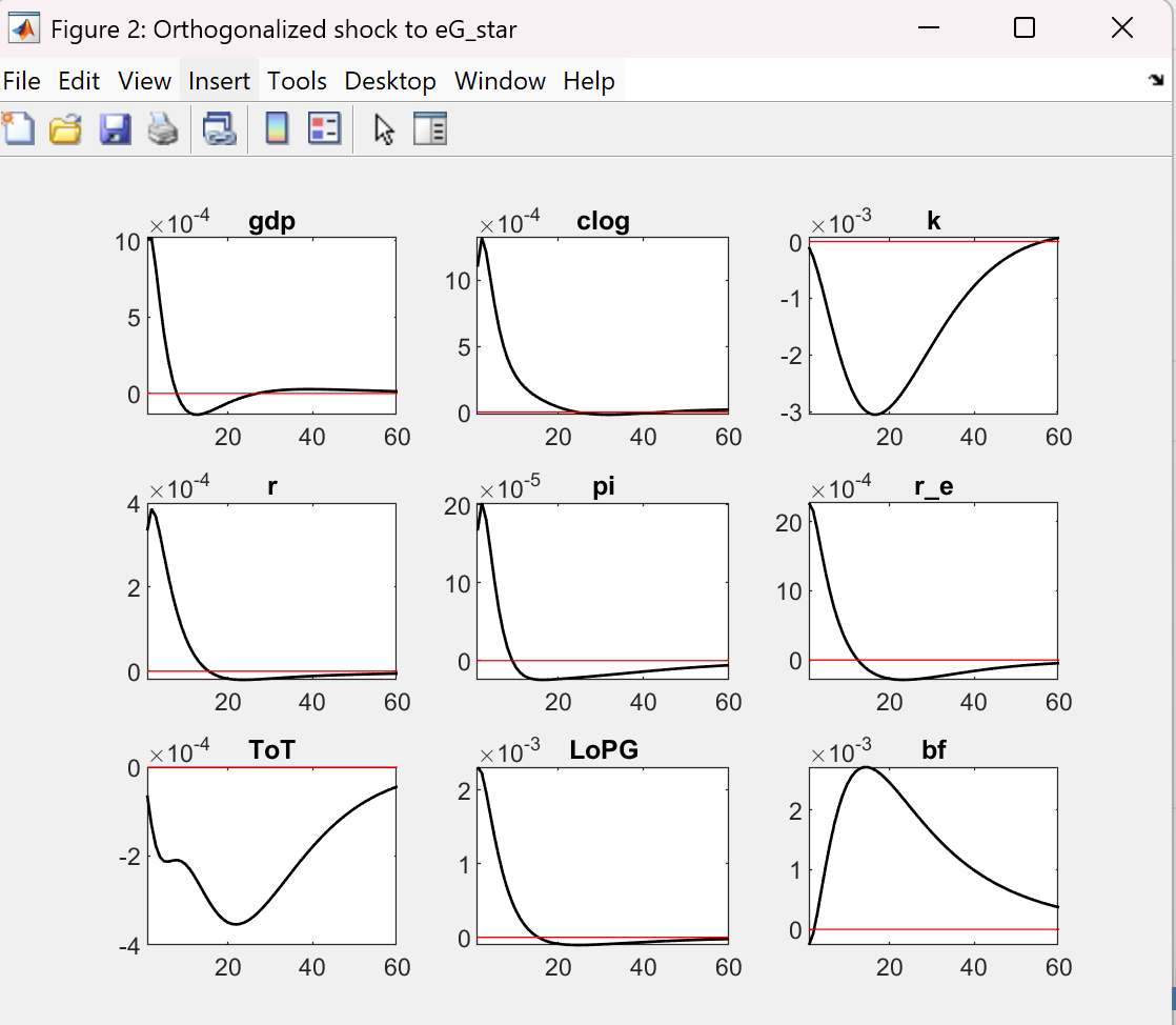
What I find “weird” in the IRFs is, for example, the behaviour of consumption following a positive tax shock (but also after foreign and technological shocks). Even after 60 periods, consumption is far from returning to its steady state (even when reducing the habit parameter), while it behaves quite standardly after other shocks. Additionally, the monetary policy response to a positive foreign shock appears unusual: it is initially positive but quickly turns negative, while the inflation reaction is negative. There are also abnormal jumps in the terms of trade.
I am actually wondering whether the integration of the open economy component has been fully and correctly modelled. Specifically, I have noticed that many linearized models include a dynamic equation for the law of one price gap. However, I cannot do this because it leads to perfect collinearity with another equation. If the dynamic model does not present any uncommon definitions, I plan to conduct a deeper analysis of the calibration, as this might explain the unusual jumps I observe.
Thank you for your guidance on this topic.
- I find the persistence not to unusual. The model has capital and you can see that the capital stock moves very persistently.
- Why is the monetary policy response strange? With a standard Taylor rule, the interest rate would follow inflation.
But yes, simplifying the model and doing sensitivity checks is usually a good idea.
In fact, I am questioning my dynamic equations, especially regarding these abnormal jumps in consumption. This might be symptomatic of calibration issues, as I had to adopt different calibrations from various papers without achieving a consistent homogenization. This challenge arises because no small open economy model with an environmental dimension currently exists with a well-calibrated framework suited to the country I am studying. I will work on this. Thank you.