Some clue about this "rank condition ISN'T verified"

I’m trying to simulate a model with three main components: transaction costs, investment adjustment costs, and Calvo price stickiness. These are my main three sources respectively: Schmitt-Grohé and Uribe (2004), Sims (2015) (which actually comes from NK’s Christiano, Eichenbaum, and Evans
(2005)) and Sims (2017) (which is a standard Calvo NK model with no capital).

When running stoch_simul() I get:

There are 6 eigenvalue(s) larger than 1 in modulus 
for 8 forward-looking variable(s)

The rank condition ISN'T verified!

From model_diagnostics:

MODEL_DIAGNOSTICS:  No obvious problems with this mod-file were detected.

I suspect that the problem might come from omitting one relevant equation by including a redundant one. My initial guess was that as I firstly set-up the mod file, there was not an explicit equation for the marginal cost mc_t, since now I have a FOC for the investment decision (from the Investment Cost part), then I combined Euler equation (3) with Investment FOC (2) through mu_t(+1), and equation (2) took the place of an explicit expression for mc_t. The steady state gets solved correctly, but I still get problems with BK conditions.

(UPDATE 2) To be more specific, the problem I see is that I have an additional FOC from HH’s problem which is: \frac{\partial L}{\partial I_t}=0, which introduces another multiplier \mu_t, and is associated with the constraint of the investment process (with adjustment costs as in CEE (2005)), and in the other hand the FOC \frac{\partial L}{\partial k_t}=0 which constitutes the Euler equation. The specific implied question is if I should combine both in an unique equation.

Also if that’s is not the root of the problem I’d be very thankful to hear some clue about it.

(Also, a weird think that I noted is that despite computing correctly the steady state, in the residual of equation (15) it’s shown a non-zero residual, why is that?)

Thanks!

UPDATE 1: Using the other implicit definition of marginal cost (that comes from the lagrange mult. corresponding to minimization problem of intermediate firms): mc_t = \frac{1}{a_t}\left(\frac{r_t}{1-\alpha}\right)^{1-\alpha}\left(\frac{w_t}{\alpha}\right)^{\alpha} I get a non-zero residual in this equation’s steady state. Then maybe this is suggesting the problem comes from here. Nevertheless, I’d still appreciate some guidance on how to involve all relevant equations when having the mentioned set-up.

PD: Note that in my model I defined: y_t(j)=a_tk_{t-1}(j)^{1-\alpha}n_t(j)^\alpha.

tc_calvo_sgu_steadystate.m (3.3 KB)
tc_calvo_sgu.mod (7.4 KB)
vI_steady.m (288 Bytes)
  1. It’s most probably a timing error. For example, your Taylor rule looks strange. Why does it only hold in expectations?
  2. There should indeed be an FOC for capital and one for investment. The multiplier on the constraint is Tobin’s q.
  3. You may want to start with a simpler version of the model, e.g. without adjustment costs.
1 Like

Thanks! Indeed Taylor rule is wrong, it was from an extrange setting that I was experimenting, but it’s meant to be a regular contemporaneous TR. I’ll try the simpler model first way. Besides, is there the necessity to include an explicit expression for total marginal costs or just the implicit lagrange multiplier in the input demands from intermediate firms are enough in the NK framework?

As long as your system is uniquely determined, there is no reason to have that explicit definition. Put differently, the explicit definition gives one additional equation and one additional variable.

1 Like

Greetings Professor Pfeifer. Using a simpler version of the model, i.e. Calvo stickiness and transaction costs, I could perform an stoch_simul() with it. Nevertheless, there’s some things I’m not able to figure out.

  1. model_diagnostics reports this:
MODEL_DIAGNOSTICS:  The Jacobian of the static model is singular
MODEL_DIAGNOSTICS:  there is 4 colinear relationships between the variables and the equations
MODEL_DIAGNOSTICS:  The presence of a singularity problem typically indicates that there is one
MODEL_DIAGNOSTICS:  redundant equation entered in the model block, while another non-redundant equation
MODEL_DIAGNOSTICS:  is missing. The problem often derives from Walras Law.

I don’t know if both messages are related, but in the colinearity part ir reports that eqs. (20), (21), (22), (23) are the ones causing the problem. This equations are just AR(1) for shocks to different variables, is this normal or it’s sign that there’s something wrong in my math?

In the other hand, the redundancy of equations, if not related with the previous issue, what could it be?

It’s worth noting that despite all these diagnostics, the stochastic simulation runs well.

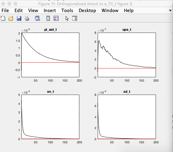
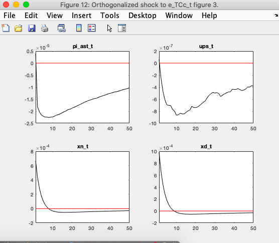
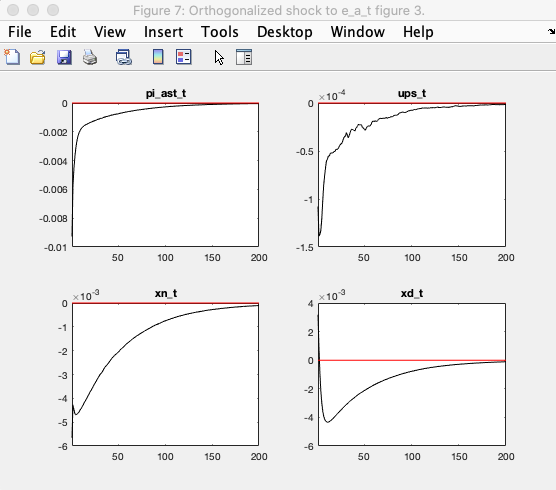
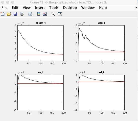
  1. For the shocks I have contemplated, I get weird irfs for price dispersion variable ups_t, since it’s too persistent and has a very noisy path:

image
image
image
image

Should I worry about that or it’s normal?

Another curious thing is that I get non-zero residual in one equation (production function) even if Dynare is able to compute the steady-state correctly, is that a bug or something?

Many thanks!
tc_calvo_cap_steadystate.m (3.3 KB)
tc_calvo_cap.mod (6.9 KB)
vI_steady.m (286 Bytes)

  1. The problem is that you are trying to use the steady_state()-operator on stuff that cannot be endogenously determined (e.g. the mean of exogenous processes). See also Levels versus Growth Rates - #8 by jpfeifer
    Hardcoding their mean to 1 resolves the collinearity:
    tc_calvo_cap.mod (6.9 KB)
  2. See
1 Like

Thanks! Actually didn’t know about that characteristic from the usage of steady_state() inside the mod file. Talking about price dispersion, just if I need a smooth irf solving for order >1, it’s necessary to set replic huge, otherwise there’s not any obvious problem with leaving it like that, right? Many thanks again!

I didn’t check whether that is sufficient, but often it is.

1 Like