Dynare noob here.
I have two questions about the interpretation of smoothed variables after an estimation (or even with calib_smoother). Suppose I have a model with output, capital, hours worked, and consumption. I feed in data for output, consumption, and hours worked, and afterwords Dynare generates smoothed capital. Is smoothed capital interpreted as deviations from its steady state? Should its plot look stationary? The smoothed variable for capital from running fs2000.mod for instance is not centered at zero and fails a Dickey Fuller test (i.e. cannot reject unit root null hypothesis).
Second, is there a mechanism by which I can generate confidence intervals for the smoothed variable? I’m thinking in terms of something like Laubach and Williams where they use a basic NK-ish type model with Kalman filters to infer the natural rate of interest and provide confidence intervals for it as well.
Thanks
Hi,
in newer Dynare version, the smoothed value contains the steady state (which may be 0 if the model is linearized). Thus, you would not expect it to be centered around 0. If your Dickey Fuller test expects a mean of 0, then you will always detect a unit root, because the process does not return to 0.
Regarding credible sets, which type of uncertainty are your estimates supposed to reflect? State uncertainty (via disturbance uncertainty) or parameter uncertainty or both? The posterior distributions produced by Dynare consider parameter uncertainty. Please also have a look at the smoothed_state_uncertainty option in the manual of 4.5.7. For a given parameter, it will provide the state uncertainty.
Thanks for the reply! Great information, as always.
Duly noted on the Dickey-Fuller test; demeaning smoothed k in fs2000.mod indeed passes the Dickey-Fuller test. My own model is giving some smoothed values that seem to grow or shrink over time. They also pass the Dickey-Fuller test when demeaned, but are visually striking nonetheless. For example, 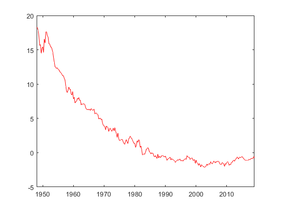
would be interpreted as a sustained period of above steady-state capital followed by a sustained period of below steady-state capital? Seems wacky, a problem with my parameterization perhaps?
Regarding state uncertainty, this looks like what I’m after, although I’m having some difficulty unpacking it. To construct the width I’m going to need the critical value via inverse normal cdf, times the standard error; but it’s not clear to me how to unpack the standard error of the kth variable in period t. Any guidance?
Thanks again.