I am simulating a ‘pre-announced favorable shock in the future’ with the following code
var eB; periods 1, 2, 3, 4, 5; values 0.5, 0.62, 0.73, 0.84, 0.95;
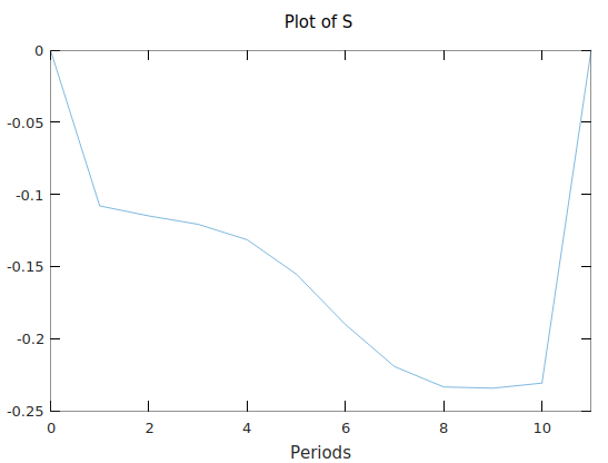
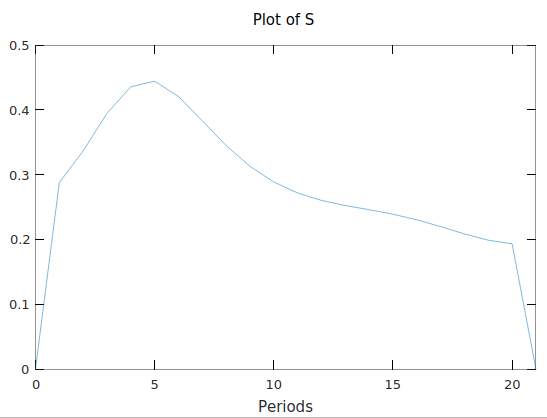
But simul(periods=10); and simul(periods=20); give different dynamics. Below is the response of variable S to the shock which is like the opposite of the other. Am I missing something, or why should the number of simulation periods matter given that it changes the entire propagation mechanism of the shock.
How do dynare users choose which period to use? Or simul(periods=5); should be the appropriate accompanying command.
Perfect foresight solutions are a two-boundary problem. Given initial and terminal conditions, you solve an equation system. But that means that you force your system to obey the terminal condition in the last period. Usually, the specified terminal condition is a steady state as a stable system will asymptotically converge back to it. But that requires you to have sufficiently many simulation periods for the system to actually return close to the terminal point.
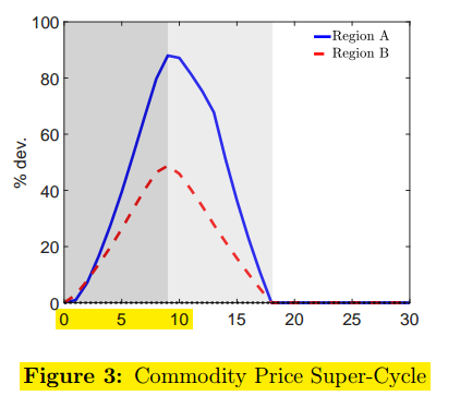
Hi Prof Pfeifer, many thanks for the reply! In the two deterministic papers I have read, the authors focus on the transmission mechanism of a given shock.
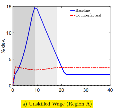
For example, here, the authors are discussing the transmission mechanism of a commodity price shock where the figure on the left is observed commodity price increase. The figure on the right is the simulated effect of the shock on unskilled wages.
So my question is
Is it that the authors, for example, use say simul(periods=500); in their code, and when reporting on the figure, they reduce the simulated sample to any number of choice? Here, 40 (in the right panel). Or they rather use simul(periods=40);? Thanks!!
My guess is that they only report the first periods of a longer simulation.