Simple NK Model Estimation with OccBin

Dear @jpfeifer and anyone who may help.

I am attempting to estimate the simplest NK model with the ZLB using OccBin but don’t get the posterior results when setting the mode_compute>0 in the estimation command. Moreover, the produced OccBin Smoothed Shocks figure seem to have a drift. I am quite sure that I am using the correct data observables to match with the model, and cannot see any apparent reason why this simple model won’t produce the estimation results.

I attach the the code and the .mat data file. I have closely followed the Atkinson et al. dynare OccBin example available on: tests/occbin/filter · master · Dynare / dynare · GitLab

Any help on how to obtain the posterior numbers using the attached code would be greatly appreciated. Thank you
NKModel.mod (6.1 KB)
Data.mat (3.3 KB)
Data2.mat (3.2 KB)

The first thing I notice is the fact that the mean of your observables differs from the steady state of the variables in the model. That will generally cause trouble.

Thank you @jpfeifer . I think I have made progress with the code and data (attached to this message). I demean the observable variables bar the interest rate, for which I use the updated shadow rate quarterly data of Wu and Xia (2016 JMCB). I don’t have the drift anymore, and it seems the model produces results and reasonable smoothed shock graphs when using mode_compute=4. Initial value of the log posterior (or likelihood): 1559.374.

I still have a few further concerns and some questions that I’ll try to make as clear as possible. Answers would be greatly appreciated:

  1. While I get posterior results, the s.d shows NaN in the prior/posterior table produced, and also NaN for the Log data density which shows just before the final graphs are produced. This occurs when I have 3 observables. However, when I remove the R_d_obs, I also retrieve estimation results with the s.d. of the posteriors showing lower values than the assumed s.d. of the priors. I am not sure how to interpret these findings, particularly the NaN when matching the 3 variables.
  2. It does take time for the model to solve with mode_check=4 but it seems to solve as mentioned. However, when using mode_check=6, the model runs for ages with the “acceptance ratio” bar not really moving? Is this normal, which posterior mode results should I show in the final estimation table (mode_check 4 or 6? the latter not working currently).
  3. I have noticed that in the Atkinson et al (2020 JME) dynare example (attached to my original message) that there is the ‘mode_file=NKM_mh_mode_saved’ in the estimation command which allows to produce posterior results under mode_compute=0, with the model solved very quickly. Where exactly do I find the mode_file corresponding with my model file so I can also use in my estimation command? Is it somewhere on the Workspace or elsewhere as I cannot seem to find it?
  4. In general, I’m confused mainly about the mode_file location and the potential difference in the posterior means produced under different mode_compute>0. Which command should be used to retrieve the true posteriors based on the model estimation?

Please let me know if you spot any other potential errors in the code and data files attached. Thank you very much in advance.

NKModelNL.mod (6.6 KB)
Data.mat (3.3 KB)
Data2.mat (3.2 KB)

  1. The DataNL.mat is missing.
  2. Yes, it’s normal that mode_compute=6 is really slow.
  3. The _mh_mode file is automatically created at the end of a MCMC run with mh_replic>0. Once you have a file like that, you can reload it without rerunning mode_compute. Without the MCMC, there will be a _mode.mat in the results subfolder.
  4. There is no general rule. With mode-finding it’s often trial and error to see whether you have found a global mode.

Thanks again @jpfeifer , I do appreciate your time. So here are my updated questions / concerns after running my code and comparing it with the Atkinson et al (2020 JME) example.

1) In both my model and the Atkinson et al. example, I set mode_compute=4 and mh_replic=400000. I try to obtain the _mode.mat file from the Atkinson et al. example without using their saved one. Running either of these models with mh_replic>0 produces on the one hand some reasonable posterior values as well as mode_check figures but fails to produce a new _mode.mat file on the other. The error message received in both models, after the posteriors and figures are produced, is:

**""**Log data density [Laplace approximation] is NaN.

Error using chol
Matrix must be positive definite.

Error in posterior_sampler_initialization (line 77)
d = chol(vv);

Error in posterior_sampler (line 60)
    posterior_sampler_initialization(TargetFun, xparam1, vv, mh_bounds,dataset_,dataset_info,options_,M_,estim_params_,bayestopt_,oo_, dispString);

Error in dynare_estimation_1 (line 432)
                posterior_sampler(objective_function,posterior_sampler_options.proposal_distribution,xparam1,posterior_sampler_options,bounds,dataset_,dataset_info,options_,M_,estim_params_,bayestopt_,oo_,dispString);

Error in dynare_estimation (line 105)
    dynare_estimation_1(var_list,dname);

Error in NKM.driver (line 947)
oo_recursive_=dynare_estimation(var_list_);

Error in dynare (line 310)
    evalin('base',[fname '.driver']);**""**

Setting mh_replic=0 and mode_compute=4 does not produce this error message but still produces NaN for the Laplace. Given that this is a shared problem with both the official example and my code, I’m not sure what could be wrong here.

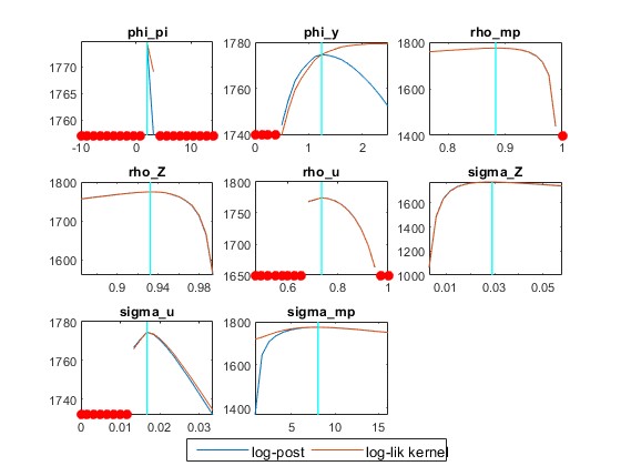
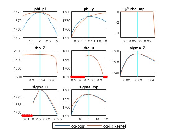
2) How important is using a 0 value for the prior_trunc? I understand that it deals with unit roots but having prior_trunc=0 or ignoring this option in the estimation command produces slightly different results, especially the mode_check figure for the inflation response in the Taylor rule that is truncated very close to its prior. Should this option be used or not in general? For example, In the Atkinson et al. example, with mode_compute=4 and mh_replic=400000, the model fails to produce the full mode check plots when ignoring prior_trunc=0.

  1. Beyond the code for my .mod model file and Data and Data 2 .mat files, which are interlinked, I attach a picture of the mode_check figure produced from my model for both prior_trunc=0 and no prior_trunc (I’m not sure why you referred to the ‘DataNL.mat’ file in the previous message?). In any case, I’m not sure how to interpret the mode_check files, especially thi phi_pi with prior_trunc=0 and the rho_mp without the prior_trunc option.

Apologies for the long message, I tried to be as elaborate and clear as possible. I hope you can point me in the right direction for my three concerns above. Thanks in advance and all the best.

NKModelNL.mod (6.6 KB)
Data.mat (3.3 KB)
Data2.mat (3.2 KB)
mode_check_priortrunc=0
mode_check_prior_trunc ignored

  1. To run the MCMC, you need a positive definite covariance matrix for the proposal distribution. By default, Dynare uses the inverse Hessian at the mode, which is not positive definite in your case. That’s what causes the error message.
  2. Corner solutions will pretty much never has a positive definite Hessian. That’s why it may be important to set prior_trunc=0. It has nothing to do with unit roots, but rather whether you allow a priori highly unlikely parameter values.
  3. The mode_check plots clearly show issues in finding the mode for phi_pi. That may explain the issue with the Hessian.