I am currently working on an small open economy DSGE model where as usual their is a combination of home and imported goods (usually investment and consumption). For policy purposes headline inflation is divided into three components:
Core Inflation (where this home and foreing goods are included)
Food Inflation
Energy Inflation (or regulated inflation)
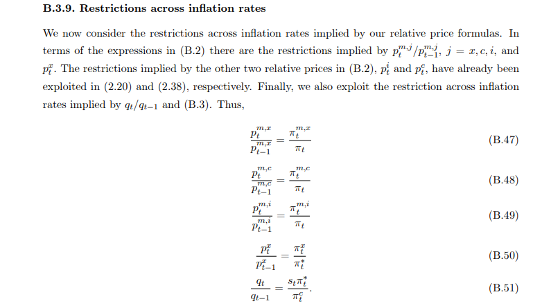
This is important because some times food and regulated prices can affect drastically headline inflation (for example during a climate phenomena like el niño). Due to the nature of food inflation and regulated inflation this variables are asume to be AR(1) processes that converges to their steady state value. In the model we asume that food and regulated inflations steady state are the same as the headline inflation and the inflation target. This is usually done. For example see the relative prices restriction in RAMSES II model:
However, the problem is that in the data this inflations are very different from the inflation target of 3%, so the AR(1) processes structure would result in large forecast errors for this variables (even just only taking into account the mean of the process).
QUESTION:
Is their any way of modeling different steady state values for this inflation components given the relative prices restrictions usually imposed in this models?
I am not sure I fully grasp the theoretical complexity here. But usually having different inflation rates implies that relative prices will diverge over time. Unless this change in relative prices is counteracted by a different mechanism, this will imply a divergence in consumption shares and therefore render the model non-stationary, i.e. there may be no steady state.
Well for example authors like Lawrence Cristiano et al (2014)AER in their paper “Risk Shocks” show how to introduce different trends for investment and consumption - GDP that implies different growth rates (as usually investment growth is higher than consumption growth). This is also related to the fact that the relative price of investment has fallen over time am i right? So it is possible to keep a balance growth path with differences in their growth rates.
However, i have never seen a paper that do this for different inflation components. As you mention this would imply that for some theoretical reason growth rates from prices from one sector are higher (or lower) than in another sector.
This problem surges from the fact that in the data from my country the inflation rates from the regulated basket have a much higher mean than the head inflation rate. This come from the fact that the government can impose high energy tariffs or high gasoline price increases.
However their is a family of semi-structural models use by the IMF that have different means for the different inflation components. Offcourse the mean average of all the components is the inflation target of 3%, but you can have a core inflation lower than 3% and a regulated inflation higher than 3% that gives you the inflation target for the headline inflation. At the same time every basket will converge to a mean close to the data.
The CMR (2014) paper is an example of what I mentioned. Due to a Cobb-Douglas production function, there is still a BGP. Investment to GDP is falling, but technology weighted investment to GDP stays constant. So there is an appropriate detrending available. The question is if something similar would work in your model.
Yes exactly in their model they include a different trend for investment and show that this is equivalent to have a declining investment to consumption relative price (which is what we observe in the data). They do this by scaling the whole model by different technologies and resulting in different growth rates. However the model asumption is that the relative prices of the rest of the goods like imported or domestic goods would be stationary and close to 0 basically (they would growth at the same rates). How can i turn my model equations to reflect that for example the imported goods relative price have fallen over time? (yes been non stationary but keeping the BGP)
No, they do not assume a BGP, but rather it is a direct result of the model features. You need to find out how that is consistent with a BGP. I doubt that is feasible. Particularly when it comes to food and energy there are non-homotheticities and decreasing energy intensities per unit of GDP at play.
When income grows, the share of food expenditures tends to go down. That renders models explicitly modeling food expenditure non-stationary.
2, We observe decreases in energy intensity per unit of GDP. That may be a similar problem.
Both items point towards some form of structural change that you are wading into when you try to model this explicitly.
So maybe what i could do is modelling the relative prices with a trend and solve the model with the difuse filter that allows non stationary models? However i dont like that approach very much because their is not a theoretical explanation of why the relative price of food has fallen over time…
That would not help. The problem is that the trends are non-uniform, so that no BGP exists. That renders Taylor approximations around a point increasing invalid over time. Estimation with perturbation techniques will then not work.