I have a question.
I want to replicate chapter 11.11 Growth RMT RMT4_ch11.pdf (540.8 KB)
So I tried to succeed to making code, but it’s failure.
Could you help me?
%-----------------------------------------------------------------------------------------------
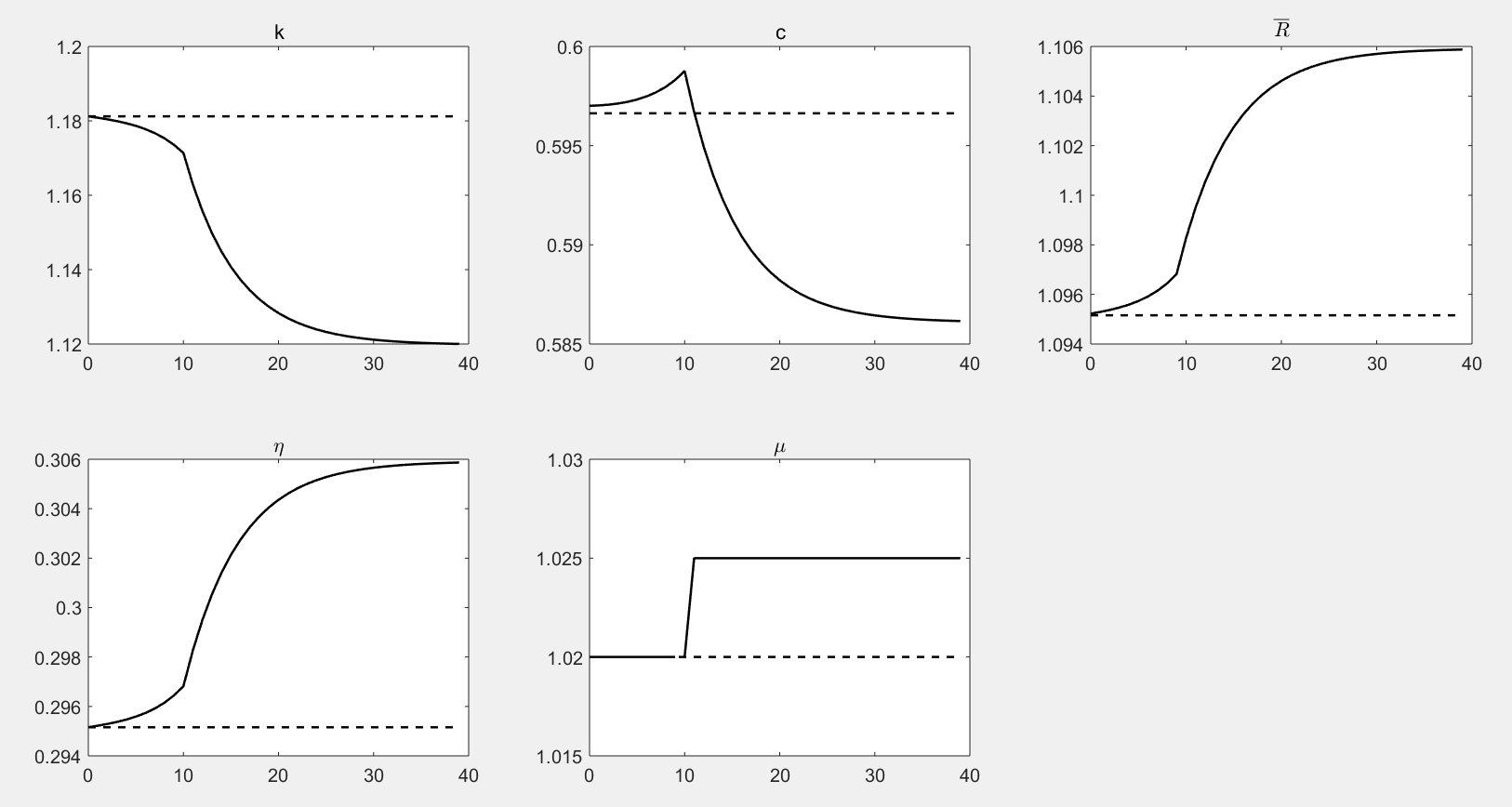
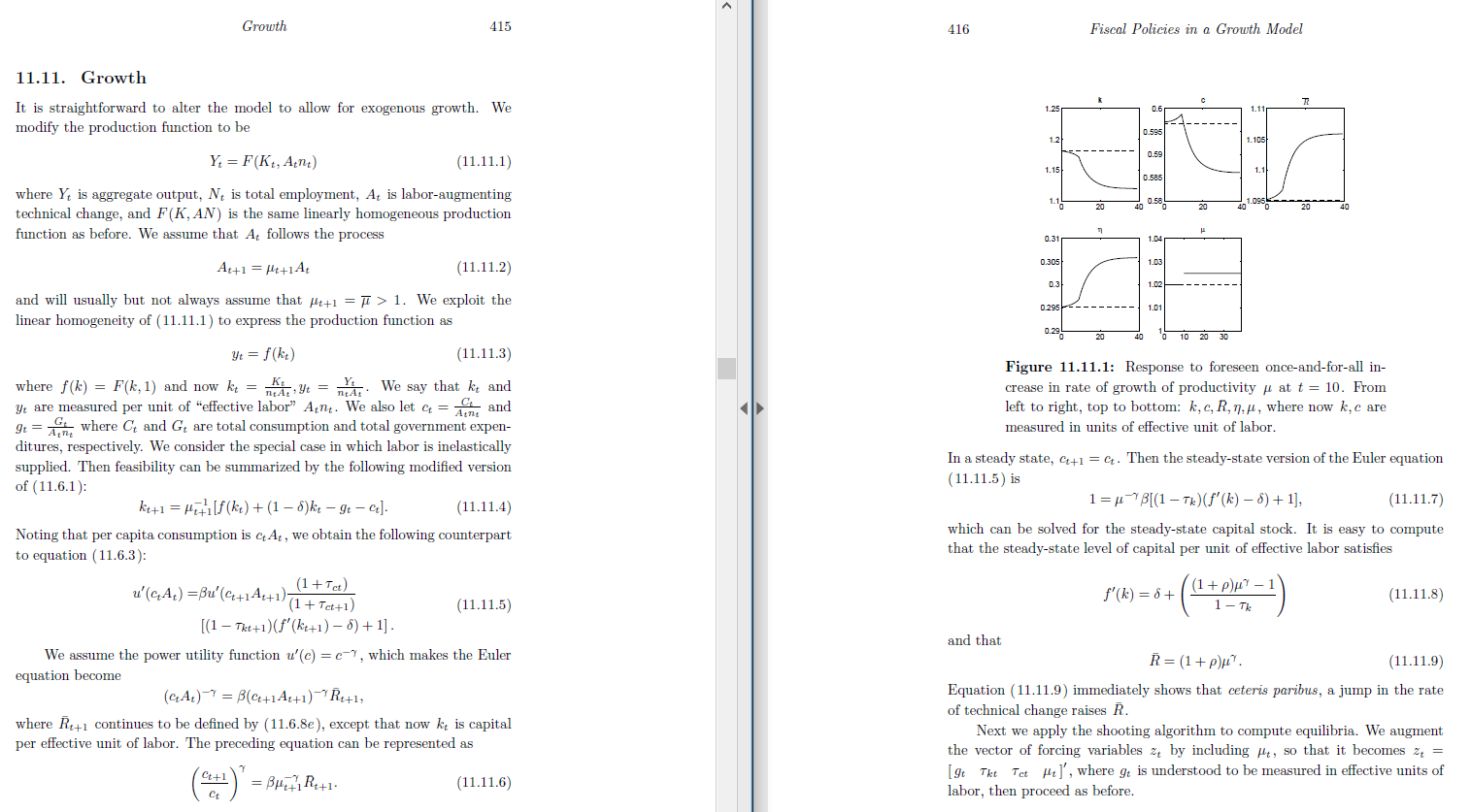
% Experiment : Permenant increase in mu at t=10
% Note:Following the discussion in the text t = 0 is the first period of the new (simulated) path
%-----------------------------------------------------------------------------------------------
// This program replicates figure 11.11.1 from chapter 11 of RMT3 by Ljungqvist and Sargent
// Dynare records the endogenous variables with the following convention.
//Say N is the number of simulations(sample)
//Index 1 : Initial values (steady sate)
//Index 2 to N+1 : N simulated values
//Index N+2 : Terminal Value (Steady State)
// Warning: we align c, k, and the taxes to exploit the dynare syntax.
//In Dynare the timing of the variable reflects the date when the variable is decided.
//For instance the capital stock for time ‘t’ is decided in time ‘t-1’(end of period).
//So a statement like k(t+1) = i(t) + (1-del)*k(t) would translate to
// k(t) = i(t) +(1-del)*k(t-1) in the code.
%-----------------------------------------------------------------------------------------------
% 1. Defining variables
%-----------------------------------------------------------------------------------------------
@#define simulation_periods=100
// Declares the endogenous variables consumption (‘c’) capital stock (‘k’) total factor productivity (‘A’);
var c k A;
// declares the exogenous variables consumption tax (‘tauc’),
// capital tax(‘tauk’), government spending(‘g’), growth rate of productivity (‘mu’)
varexo tauc tauk g mu;
parameters bet gam del alpha;
%-----------------------------------------------------------------------------------------------
% 2. Calibration and alignment convention
%-----------------------------------------------------------------------------------------------
bet=.95; // discount factor
gam=2; // CRRA parameter
del=.2; // depreciation rate
alpha=.33; // capital’s share
// Alignment convention:
// g tauc tauk are now columns of ex_. Because of a bad design decision the date of ex_(1,
// doesn’t necessarily match the date in endogenous variables. Whether they match depends on
// the number of lag periods in endogenous versus exogenous variables.
// These decisions and the timing conventions mean that
// k(1) records the initial steady state, while k(102) records the terminal steady state values.
// For j > 1, k(j) records the variables for j-1th simulation where the capital stock decision
// taken in j-1th simulation i.e stock at the beginning of period j.
// The variable ex_ also follows a different timing convention i.e
// ex_(j, records the value of exogenous variables in the jth simulation.
// The jump in the government policy is reflected in ex_(11,1) for instance.
%-----------------------------------------------------------------------------------------------
% 3. Model
%-----------------------------------------------------------------------------------------------
model;
// equation 11.11.2
A=1*(1+mu)^(@{simulation_periods}+1);
// equation 11.11.4
k=(A*k(-1)^alpha+(1-del)*k(-1)-c-g)/mu;
// equation 11.11.6
c^(-gam)= bet*(c(+1)^(-gam)mu^(-gam))((1+tauc)/(1+tauc(+1)))((1-del) + (1-tauk(+1))alphaAk^(alpha-1));
end;
%-----------------------------------------------------------------------------------------------
% 4. Computation
%-----------------------------------------------------------------------------------------------
initval;
k=1.5;
c=0.6;
g = .2;
tauc = 0;
tauk = 0;
mu=0.02;
A=1*(1+mu)^0;
end;
// put this in if you want to start from the initial steady state,comment it out to start
// from the indicated values
// The following values determine the new steady state after the shocks.
endval;
k=1.5;
c=0.6;
g =.4;
tauc =0;
tauk =0;
mu=0.025;
A=1*(1+mu)^(@{simulation_periods}+1);
end;
// We use ‘steady’ again and the endval provided are initial guesses for dynare to compute the ss.
// The following lines produce a g sequence with a once and for all jump in g
// we use ‘shocks’ to undo that for the first 10 periods (t=0 until t=9)and leave g at
// it’s initial value of 0
// Note : period j refers to the value in the jth simulation
shocks;
var mu;
periods 1:10;
values 0.02;
end;
// now solve the model
simul(periods=100);
// Compute the initial steady state for consumption to later do the plots.
c0=c(1);
k0 = k(1);
// g is in ex_(:,1) since it is stored in alphabetical order
g0 = ex0_(3)
A0=1;
%-----------------------------------------------------------------------------------------------
% 5. Graphs and plots for other endogenous variables
%-----------------------------------------------------------------------------------------------
// Let N be the periods to plot
N=40;
// The following equation compute the other endogenous variables use in the plots below
// Since they are function of capital and consumption, so we can compute them from the solved
// model above.
// These equations were taken from page 371 of RMT3
rbig0=1/bet;
rbig=c(2:101).^(-gam)./(betc(3:102).^(-gam));
nq0=alphaA0k0^(alpha-1);
nq=alphaA(1:100).k(1:100).^(alpha-1);
wq0=A0k0^alpha-k0alphaA0*k0^(alpha-1);
wq=A(1:100).*k(1:100).^alpha-k(1:100).*alpha.*A(1:100).*k(1:100).^(alpha-1);
// Now we plot the responses of the endogenous variables to the shock.
x=0:N-1;
figure(1)
// subplot for capital ‘k’
subplot(2,3,1)
plot(x,[k0*ones(N,1)],’–k’, x,k(1:N),‘k’,‘LineWidth’,1.5)
// note the timing: we lag capital to correct for syntax
title(‘k’,‘Fontsize’,12)
set(gca,‘Fontsize’,12)
// subplot for consumption ‘c’
subplot(2,3,2)
plot(x,[c0*ones(N,1)],’–k’, x,c(2:N+1),‘k’,‘LineWidth’,1.5)
title(‘c’,‘Fontsize’,12)
set(gca,‘Fontsize’,12)
// subplot for cost of capital ‘R_bar’
subplot(2,3,3)
plot(x,[rbig0*ones(N,1)],’–k’, x,rbig(1:N),‘k’,‘LineWidth’,1.5)
title(’\overline{R}’,‘interpreter’, ‘latex’,‘Fontsize’,12)
set(gca,‘Fontsize’,12)
// subplot for rental rate ‘eta’
subplot(2,3,4)
plot(x,[nq0*ones(N,1)],’–k’, x,nq(1:N),‘k’,‘LineWidth’,1.5)
title(’\eta’,‘Fontsize’,12)
set(gca,‘Fontsize’,12)
// subplot for the experiment proposed
subplot(2,3,5)
plot([0:9],1 + oo_.exo_simul(1:10,4),‘k’,‘LineWidth’,1.5);
hold on;
plot([10:N-1],1 + oo_.exo_simul(11:N,4),‘k’,‘LineWidth’,1.5);
hold on;
plot(x,[g0*ones(N,1)],’–k’,‘LineWidth’,1.5)
title(‘mu’,‘Fontsize’,12)
axis([0 N -.1 .5])
set(gca,‘Fontsize’,12)
print -depsc fig_g.eps