I am currently trying to replicate the paper “Modeling the Liquidity Effect of a Money Shock” by Christiano (1991) . For the replication I use a simplified version and abstract from the labor augmenting technological process mu, so that I only have growth in nominal variables. This is done since I am mainly interested about the effects of the money shock.
After solving for the first order conditions, deflating all the nominal variables, computing the steady state and log-linearizing the model, I run into some issues in my dynare code.
Unfortunately, the simulation yields a violation of the Blanchard-Kahn condition.
There are 2 eigenvalue(s) larger than 1 in modulus
for 4 forward-looking variable(s)
Replacing the Euler Equation in the dynare code by the third FOC from the household (which is commented out in the code), allows the code to run. However, the obtained IRFs with respect to the money shock (x) are not equal to the ones provided in the original paper. I think, that using the Euler Equation should solve the problem, however, I cannot get it to run.
Plugging in for the concrete utility function which is (1-\gamma) log (C_t) + \gamma *log(1-L_t)
helps to cancel the marginal utility term, since in the absence of real growth c_t is constant.
Deflating the retrieved expression for the nominal growth which is caused by the money shock and thus divide
all nominal variables in period t by M_t. By simplifying and replacing (M_{t+1} / M_t) by the growth rate of money (1+x) I obtain the Euler Equation given in the .mod file after log-linearizing all the equations.
Thank you for your response.
In the meanwhile I was able to figure out the problems with the Blanchard-Kahn condition in the code posted above.
However, when trying to implement the extension of Fuerst-Lucas, where households have to take their loan decision before they know about the shock and thus implementing the EXPECTATION(-1) operator in my code, I get a strange error.
It says the Blanchard-Kahn conditions are violated, even though the # of Eigenvalues > 1 = # Forward Looking variables. This happens, no matter wheter I use (1+xt) or (1+xt(+1)) as you suggested before.
Do you perhaps know, what the problem is when this message occurs?
What was the issue with the first file? Did you replicate the results of the paper?
Are you sure the timing is correct. For example, you have EXPECTATION(-1)((gamma/(1-exp(l)))) but l is chosen today by the household and should be known.
Concerning 1)
The issue in the first file was, that I missed a term when deriving the FOC of the firm. I added this term and then it worked. The IRFs I retrieve from Dynare match perfectly with the ones from the paper.
Concerning 2)
You are right that the timing convention was not for the equation you mentioned.
The timing convention I used stems from the paper, from the following equation:
Thus, the EXPECTATION(-1) should only pertain to the Euler Equation.
I was able to replicate the results from the paper, but only by excluding the interest rate from EXPECTATION(-1) in the Euler Equation.
While the results look nice, I fail to grasp the intuition for understanding which variables should be included in the EXPECTATION(-1) and which variables should not be included.
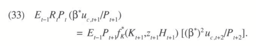
This poses a further problem for the 2nd extension (Sluggish-Capital Model) of the Model done by Christiano, which also makes the firm decide on their investment in period t-1, before the shock is known, which yields the following FOC for the firm wrt to capital:
I tried to implement it, again using the EXPECTATION(-1) , however only for capital, prices and the shocks, as I think that consumption is decided at the respective time again, and without expectation.
That is strange. The paper should specify which decisions are taken with which information set. Note that you may have to shift the whole equation (31) by one period in Dynare . The convention is to specify how variables at time t are decided, but the equation above links time t-1 variables (as E_{t-1} is a time t-1 variable).
I really appreciate your help. Your comment on the timing convention allowed me to finally replicate the results of the paper by shifting the whole expression by 1 period.
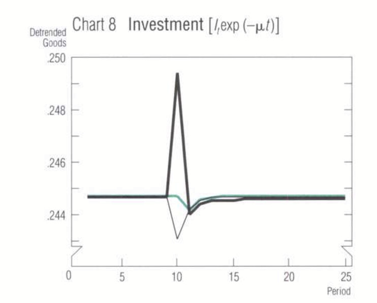
There is only one thing that puzzles me which has to do with the interpretations of the IRFs. All the IRFs look perfectly fine in the model with Sluggish capital, except for the one for investment.
The original IRF on the right (the green line) remains constant at the period of the shock (since capital is sluggish and firms can only change investment for period t+1 at period t.
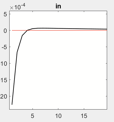
However, in the IRFs I obtain from Dynare, investment starts already below the initial level.
Upon zooming in I noticed that the plot of the IRF starts at period 1 and not period 0.
Can I interpret this in this way that the IRF of Dynare does not plot the period of the shock t=0, and instead just shows the first period after the shock which is t+1 and where firms were already able to adjust their investment or am I missing something here?
I am not sure I understand the question. Dynare will report IRFs so that the period the shock happens is at time 1. But your question seems concerned with the timing of predetermined variables. Dynare will generally report variables using the standard timing. So if you have
exp(in(-1)) = exp(k) - (1-delta)*exp(k(-1)); // law of motion capital
then Dynare’s IRFs will report in, which moves at time t but will only add to k(+1).