Hi Dynare experts,
I would like to study the response of a set of variables to a shock (e.g. demand shock) in two regimes:
- high output volatility,
- low output volatility.
Could you please tell me if I can do this in Dynare? and how?
Thank you.
Hi Dynare experts,
I would like to study the response of a set of variables to a shock (e.g. demand shock) in two regimes:
Could you please tell me if I can do this in Dynare? and how?
Thank you.
What exactly are you trying to do? Please describe the modeling environment you have in mind. You want a regime-switching DSGE model?
Dear Johannes,
Thank you for your prompt answer and apologies for being vague on my side.
Yes, the environment is a DSGE model. Let me be more clear: Take for example the baseline RBC model (code on your website): github.com/JohannesPfeifer/DSGE … seline.mod
In this model, there are two shocks: a shocks to TFP and a government spending shock.
What I would like to do is to augment the TFP with a time-varying volatility shock. Then, I can parameterize the shock such that I get regime 1) high time-varying volatility, regime 2) low time-varying volatility. Then, I would like to see how model variables, in particular output, would respond differently to government expenditure shocks in times of high and low volatility.
Would that be feasible? My concern is that it may not be because, according to my understanding, when there are two shocks and we study the responses of variables to the shocks, we get first the responses of variables to one shock while the other one is muted and then the other way around. Am I right?
Would there be any other way to study in this kind of DSGE setup the response of model variables to government spending shocks in times of high versus low output volatility?
Hope this is clear; if not please let me know. I would very much appreciate your help. Thank you.
So if I understand you would have first to add a third shock on the variance of the innovation of the TFP.
You cannot do that with a first order approximation of the model (as in the example, posted by Johannes, you give as a reference). Even with a second order approximation, we know that the size of the shocks does not affect the slopes of the reduced form (but only the constant), so you would have at least to work with a third order approximation. With a third order approximation the size of the shocks will affect the elasticities.
Your understanding of the IRFs in Dynare is correct. That said, you could implement that by modifying the irf.m Matlab function in Dynare (you would just have to change the call to the simult_ routine). But I do not understand how you model high and low volatility regimes. Is is just a shift on a constant in the equation for the shock on the variance of the TFP? If so, why do you need to add some noise on this shock?
Best,
Stéphane.
Hi,
as Stéphane said, you need to specify the precise experiment you have in mind. Of course, as usual in the literature if you use a stochastic volatility process, you need to approximate the model at third order. In this case, the IRFs are actually Generalized IRFs. Thus, you need to think about both the point in the state-space at which you construct the IRFs as well as the general stochastic properties. If your two regimes are just characterized by a different shock standard deviation for the volatility shock (high vs. low time-varying volatility), then you can just run the mod-file twice for different values of the standard deviation of the volatility shock in the shocks-block. However, I guess what you actually have in mind is having a fixed standard deviation of this volatility shock in both experiments, but looking at the government spending shock IRF for a case where the volatility state is high vs low (i.e. it was preceeded by a high/low volatility shock). In this case, you would need to use the simult_-function to construct the particular simulations. An example for using this function is at sites.google.com/site/pfeiferec … edirects=0 shows how to compute GIRFs.
Dear Johannes, dear Stephane,
Thank you both very much for your suggestions and advice. They were extremely helpful and I made progress, but I haven’t resolved my problem, yet.
For clarity, I am attaching the mod file (see below), which contains the code for the RBC model with a government spending shock and a TFP shock (very similar to https://github.com/JohannesPfeifer/DSGE_mod/blob/master/RBC_baseline/RBC_baseline.mod). I have augmented the model by introducing a time varying volatility shock on the TFP shock, which is supposed to capture the different states of high vs. low time of uncertainty. This regime switching I model by imposing a different value for the standard deviation of the time-varying volatility shock.
From the model, I want to understand how output (y) responds to government expenditure shocks in times of high vs. times of low uncertainty. To get this, what I have in mind is to calculate IRFs of output (y) (or GIRFs, not sure which would be the correct one) in response to government expenditure shocks, but taking into account the state, which is determined by the time-varying volatility on the TFP shock, i.e. (1) the standard deviation of the time-varying volatility is high (high uncertainty state), and when (2) it is low (low uncertainty state). I tried following the codes that Johannes suggested, but all of this is new to me and I still cannot figure out the solution. I have the following questions:
The Generalized IRFs represent the responses of the variables that take into account all shocks, not government expenditure shocks alone. Am I right? And if so, is there any way that I can have the responses of the variables only to government expenditure shocks, but taking into account that there is a high and low uncertainty environment?
The code by Johannes used to calculate GIRFs (https://sites.google.com/site/pfeiferecon/RBC_state_dependent_GIRF.mod?attredirects=0) specifies positive and negative value for the volatility for the government expenditure shock in the part where it is calculating the GIRFs. But the volatility of the government shock is defined also in the shock block earlier. Then, I don’t understand what is the shock value that is applied to the government expenditure shock in the simulations?
If you have any other suggestions on how to get what I described earlier, I would be extremely grateful.
Apologies for the long email and questions. Hope you can help me out. It will be very much appreciated.
king_rebelo2.mod (10.5 KB)
The GIRFs consider the impulse response to one particular shock, while averaging out all other shocks. This is important, because at higher order the IRFs are state-dependent. Because of this, future shock realizations will impact the IRF path. One way to get around specifying a particular shock path is to simply integrate these shocks out.
In my GIRF code, you would have to keep the shock size for the G shock fixed at a positive one for both cases. What you would have to change is the value for the volatility state at which this shock happens. What you need to distinguish to understand what is going on is the shock realization for the IRFs and the shock distribution from which it is drawn from. You need to specify both. The shock distribution is specified in the shocks-block. The shock size for the IRF is given in the shock matrix fed into the simult_-function
Dear Johannes,
Thank you so much for all your help. Highly appreciated. Unfortunately, I still cannot produce the results I want. Couple of issues:
In your code (https://sites.google.com/site/pfeiferecon/RBC_state_dependent_GIRF.mod?attredirects=0), you define shocks_baseline and shocks_impulse. What is the purpose of the shocks_baseline? If I just want to calculate the GIRFs of output to a government expenditure shock, do I need to have in the IRF_mat only (y_shock) or the difference (y_shock-y_baseline)?
Following your suggestions and if my understanding is correct, I specified the size of the government shock in the part where I calculate the GIRFs (setting it equal to 1). Then, when I change the value of the variance of the volatility shock in the shock block (i.e. the shock distribution), the simulated series are almost the same regardless if the value of the volatility shock is high or low. The simulated series can be accessed in the matlab folder GIRF_positive (I am following the names of your original code). Is that correct? If so, I don’t know what I am doing wrong to be getting the same simulations regardless of the shock distribution I specify. I am attaching my code.
Thank you in advance!
king_rebelo3.mod (8.1 KB)
If I understand you correctly, you want something like the following
/*
 * This file presents a baseline RBC model with TFP and government spending shocks, calibrated to US data from
 *  1947Q4:2016Q1. The model setup is described in Handout_RBC_model.pdf and resembles the one in King/Rebelo (1999):
 *  Resuscitating Real Business Cycles, Handbook of Macroeconomics, Volume 1 and
 *  Romer (2012), Advanced macroeconomics, 4th edition
 *  The driving processes are estimated as AR(1)-processes on linearly detrended data.
 *
 * This implementation was written by Johannes Pfeifer. In case you spot mistakes,
 * email me at jpfeifer@gmx.de
 *
 * Please note that the following copyright notice only applies to this Dynare
 * implementation of the model.
 */

/*
 * Copyright (C) 2016 Johannes Pfeifer
 *
 * This is free software: you can redistribute it and/or modify
 * it under the terms of the GNU General Public License as published by
 * the Free Software Foundation, either version 3 of the License, or
 * (at your option) any later version.
 *
 * It is distributed in the hope that it will be useful,
 * but WITHOUT ANY WARRANTY; without even the implied warranty of
 * MERCHANTABILITY or FITNESS FOR A PARTICULAR PURPOSE.  See the
 * GNU General Public License for more details.
 *
 * For a copy of the GNU General Public License,
 * see <http://www.gnu.org/licenses/>.
 */

//****************************************************************************
//Define variables
//****************************************************************************

var y c k l z ghat r w  invest vol log_y log_k log_c log_l log_w log_invest;
varexo eps_z eps_g omega;

//****************************************************************************
//Define parameters
//****************************************************************************

parameters beta psi sigma delta alpha rhoz rhog gammax rho vol_bar eta
    gshare n x i_y k_y g_ss;

//****************************************************************************
//Set parameter values
//****************************************************************************

sigma=1;                // risk aversion
alpha= 0.33;            // capital share
i_y=0.25;               // investment-output ration
k_y=10.4;               // capital-output ratio
x=0.0055;               // technology growth (per capita output growth)
n=0.0027;               // population growth
rhoz=0.97;              //technology autocorrelation base on linearly detrended Solow residual
rhog=0.989;
gshare=0.2038;          //government spending share
rho=0.9;                 //persistance of volatility
vol_bar = log(0.021);
eta = 0.06;

//****************************************************************************
//enter the model equations (model-block)
//****************************************************************************

model;
[name='Euler equation']
c^(-sigma)=beta/gammax*c(+1)^(-sigma)*
    (alpha*exp(z(+1))*(k/l(+1))^(alpha-1)+(1-delta));
[name='Labor FOC']
psi*c^sigma*1/(1-l)=w;
[name='Law of motion capital']
gammax*k=(1-delta)*k(-1)+invest;
[name='resource constraint']
y=invest+c+g_ss*exp(ghat);
[name='production function']
y=exp(z)*k(-1)^alpha*l^(1-alpha);
[name='real wage/firm FOC labor']
w=(1-alpha)*y/l;
[name='annualized real interst rate/firm FOC capital']
r=4*alpha*y/k(-1);
[name='exogenous TFP process']
z=rhoz*z(-1)+exp(vol)*eps_z;
[name='government spending process']
ghat=rhog*ghat(-1)+eps_g;
[name='volatility process']
vol=(1-rho)*vol_bar+rho*vol(-1)+eta*omega;
[name='Definition log output']
log_y = log(y);
[name='Definition log capital']
log_k = log(k);
[name='Definition log consumption']
log_c = log(c);
[name='Definition log hours']
log_l = log(l);
[name='Definition log wage']
log_w = log(w);
[name='Definition log investment']
log_invest = log(invest);

end;

//****************************************************************************
// Provide steady state values and calibrate the model to steady state labor of 0.33,
// i.e. compute the corresponding steady state values
// and the labor disutility parameter by hand;
//****************************************************************************

steady_state_model;
    //Do Calibration
    vol=vol_bar;
    gammax=(1+n)*(1+x);
    delta=i_y/k_y-x-n-n*x;
    beta=(1+x)*(1+n)/(alpha/k_y+(1-delta));
    l=0.33;
    k = ((1/beta*(1+n)*(1+x)-(1-delta))/alpha)^(1/(alpha-1))*l;
    invest = (x+n+delta+n*x)*k;
    y=k^alpha*l^(1-alpha);
    g=gshare*y;
    g_ss=g;
    c = (1-gshare)*k^(alpha)*l^(1-alpha)-invest;
    psi=(1-alpha)*(k/l)^alpha*(1-l)/c^sigma;
    w = (1-alpha)*y/l;
    r = 4*alpha*y/k;
    log_y = log(y);
    log_k = log(k);
    log_c = log(c);
    log_l = log(l);
    log_w = log(w);
    log_invest = log(invest);
    z = 0;
    ghat =0;
end;

//****************************************************************************
//set shock variances
//****************************************************************************

shocks;
    var eps_z=1;
    var eps_g=0.0104^2;
    var omega=1;
end;

//****************************************************************************
//check the starting values for the steady state
//****************************************************************************

resid;

//****************************************************************************
// compute steady state given the starting values
//****************************************************************************

steady;
//****************************************************************************
// check Blanchard-Kahn-conditions
//****************************************************************************

check;

%----------------------------------------------------------------
% compute policy function at second order
%----------------------------------------------------------------

stoch_simul(order=3,pruning,periods=0,irf=0,nofunctions);


%%%%%%%%%%%%%%%%%% Generate GIRF with positive 1% shock at ergodic mean %%%%

%define options
irf_periods=20; %IRF should have 20 periods
drop_periods=0; %drop 0 periods in simulation as burnin
irf_replication=1000; %take GIRF average over 1000 periods


%%%%%%%%%%%%%%%%%% Generate GIRF at different volatility states %%%%

impulse_vec=zeros(1,M_.exo_nbr); %initialize impulse vector to 0
impulse_vec(strmatch('eps_g',M_.exo_names,'exact'))=0.01; %impulse of minus 1 percent to g

starting_point_low=oo_.dr.ys; %define starting point of simulations; here: start at steady state
starting_point_low(strmatch('vol',M_.endo_names,'exact'))=...
    log(0.5*exp(starting_point_low(strmatch('vol',M_.endo_names,'exact')))); %set volatility to 50% below steady state
starting_point_high=oo_.dr.ys; %define starting point of simulations; here: start at steady state
starting_point_high(strmatch('vol',M_.endo_names,'exact'))=...
    log(1.5*exp(starting_point_high(strmatch('vol',M_.endo_names,'exact')))); %set volatility to 50% above steady state

%% initialize shock matrices to 0
shocks_baseline = zeros(irf_periods+drop_periods,M_.exo_nbr); %baseline
shocks_impulse = shocks_baseline;

%%  eliminate shocks with 0 variance
i_exo_var = setdiff([1:M_.exo_nbr],find(diag(M_.Sigma_e) == 0 )); %finds shocks with 0 variance
nxs = length(i_exo_var); %number of those shocks
chol_S = chol(M_.Sigma_e(i_exo_var,i_exo_var));%get Cholesky of covariance matrix to generate random numbers

IRF_mat_low=NaN(M_.endo_nbr,irf_periods,irf_replication);
IRF_mat_high=NaN(M_.endo_nbr,irf_periods,irf_replication);
for irf_iter = 1: irf_replication
    shocks_baseline(:,i_exo_var) = randn(irf_periods+drop_periods,nxs)*chol_S; %generate baseline shocks
    shocks_impulse = shocks_baseline; %use same shocks in impulse simulation
    shocks_impulse(drop_periods+1,:) = shocks_impulse(drop_periods+1,:)+impulse_vec; %add deterministic impulse
    y_baseline_low = simult_(starting_point_low,oo_.dr,shocks_baseline,options_.order); %baseline simulation
    y_shock_low = simult_(starting_point_low,oo_.dr,shocks_impulse,options_.order); %simulation with shock
    IRF_mat_low(:,:,irf_iter) = (y_shock_low(:,M_.maximum_lag+drop_periods+1:end)-y_baseline_low(:,M_.maximum_lag+drop_periods+1:end)); %add up difference between series
    y_baseline_high = simult_(starting_point_high,oo_.dr,shocks_baseline,options_.order); %baseline simulation
    y_shock_high = simult_(starting_point_high,oo_.dr,shocks_impulse,options_.order); %simulation with shock
    IRF_mat_high(:,:,irf_iter) = (y_shock_high(:,M_.maximum_lag+drop_periods+1:end)-y_baseline_high(:,M_.maximum_lag+drop_periods+1:end)); %add up difference between series
end
GIRF_high_vola=mean(IRF_mat_high,3); %take average
GIRF_low_vola=mean(IRF_mat_low,3); %take average


figure('Name','GIRFs to positive G shock')
subplot(2,1,1)
plot(1:irf_periods,GIRF_high_vola(strmatch('ghat',M_.endo_names,'exact'),:),'b-')
hold on
plot(1:irf_periods,GIRF_low_vola(strmatch('ghat',M_.endo_names,'exact'),:),'r--')
title('G')
subplot(2,1,2)
plot(1:irf_periods,GIRF_high_vola(strmatch('log_y',M_.endo_names,'exact'),:),'b-')
hold on
plot(1:irf_periods,GIRF_low_vola(strmatch('log_y',M_.endo_names,'exact'),:),'r--')
title('Y')
legend('High TFP Volatility','Low TFP volatility')
The purpose of the baseline is to have a comparison between a series with shock and one without. That is the concept of the GIRF. You need
y_shock-y_baseline
if your series are in logs to get the percentage Impulse Response.
Hi Johannes,
Thank you so much for the code and sincere apologies for getting back with such a delay, but I got caught up with other things at work.
I think this code is exactly what I am after, however, I am puzzled since it produces NO difference between the responses to G when starting at a high or a low value of volatility. Please see the result below. 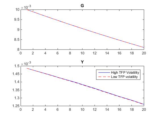
I wonder why this is the case?
When I repeat the exercise by changing the starting point of the TFP shock (z) instead of the volatility shock (vol) (i.e. changing vol to z in the starting_point in the code), I get the graph below. However, this is not what I am after since in this case the results would be interpreted as the response to G in times of high vs. low TFP; and I need the results for the responses to G in times of high vs. low volatility. 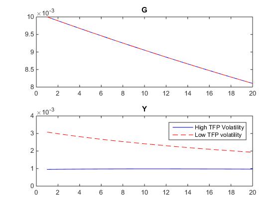
As a reminder of what I am after: I want to see how government multipliers change in times of high versus low uncertainty.
Thank you so much for all your help. All the best.
My guess is that the reason is that decision rules are close to linear in volatility as it is the g_{x\sigma\sigma} term that drives most of the effects. As a consequence, the state of volatility will not matter much for the IRFs to level shocks.
Many thanks, Johannes. I just want to clarify something.
Suppose there are two exact economies that only differ in the variance specified in the shock block. More specifically:
Economy 1:
shocks;
var eps_z=0.66^2;
var eps_g=1.04^2;
end;
Economy 2:
shocks;
var eps_z=1.2*0.66^2;
var eps_g=1.04^2;
end;
where eps_z stands for a TFP shock and eps_g stands for a government expenditures shock. As before, I want to study the responses of the variables to a government expenditure shock.
Thank you for your time and help.
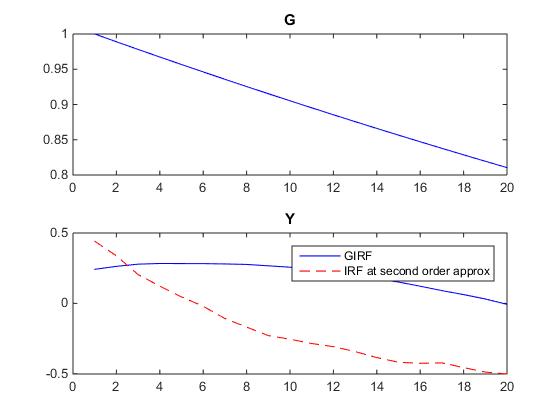
Thank you, Johannes. You mentioned that the IRFs at second order are already GIRFs. However, when I use the code attached, this is not what I get. I get the following IRFs and GIRFs for log_y in response to a shock in G. I wonder why they differ? Thank you.
king_rebelo8.mod (7.8 KB)
Hi Johannes,
I am following up on the question I posed earlier. It would be great if you could clarify this for me.
To quickly remind you, what I didn’t understand was: Why the IRFs produced by Dynare at second order approximation differ from the GIRFs produced using your code (attached in my last post)?
Thank you very much for your help.
They differ, because they are two different types of GIRFs. The ones you did manually condition the past state to be the deterministic steady state. The ones Dynare generates by default average out the initial condition, i.e. they are conducted at the ergodic mean.
Thanks a lot, Johannes.