Hi Professor,
I have got a few questions regarding the setup of SW(07) paper.
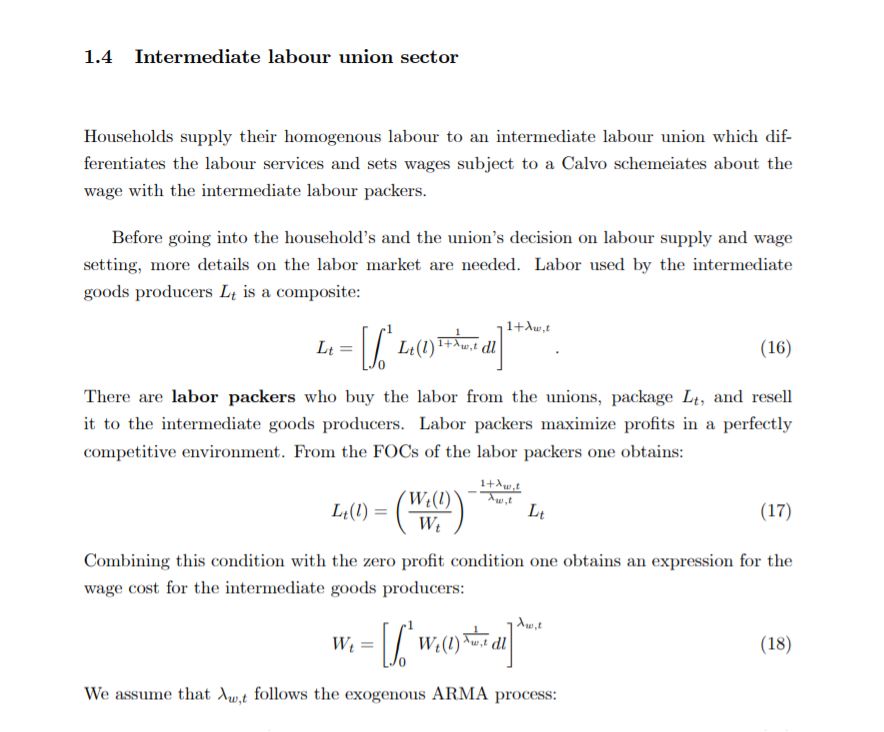
( see figure "aggregator) The paper mentions that in SW (07), the Dixit-Stiglitz aggregator in the intermediate goods and labour market is replaced by the more general aggregator developed in Kimball (1995). However, there is an online appendix which assumes the following aggregator for the intermediate goods producers which still looks like a Dixit-Stiglitz . Is there a contradiction?
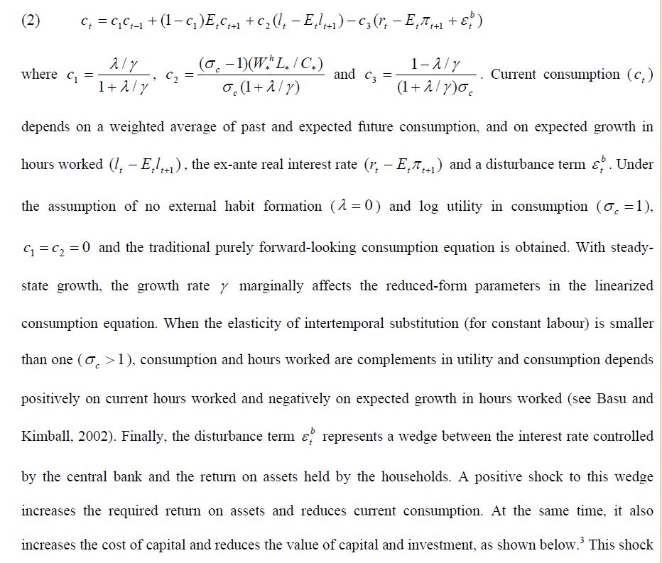
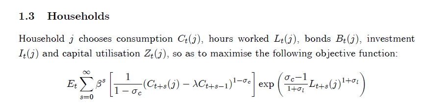
(see figure “consumption”). In the househoods utility function, the parameter “sigma_c” (inverse of the elasticty of intertemporal substitution for constant labour ) is greater than 1. This however means households would enjoy working more hours and supplying labour indefinitely? I suppose SW(07) assumes that the labour in the current period brings utility whereas the labour in the next period brings disutility? Please could you confirm my understanding?
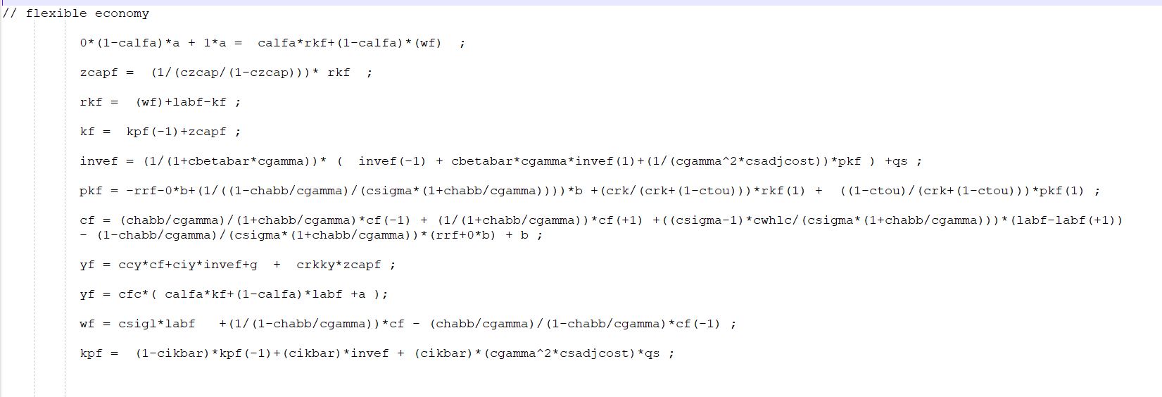
( see figure “sticky and flexible”). From the dynare code, it seems that to derive the flexible version, the MC ( negative price markup, - \mu^p_t) is set to 0, and then we solve for rental rate of capital rk_t from it). My question is, how to derive the inflation for the flexible economy? there is no equation for inflation for it.
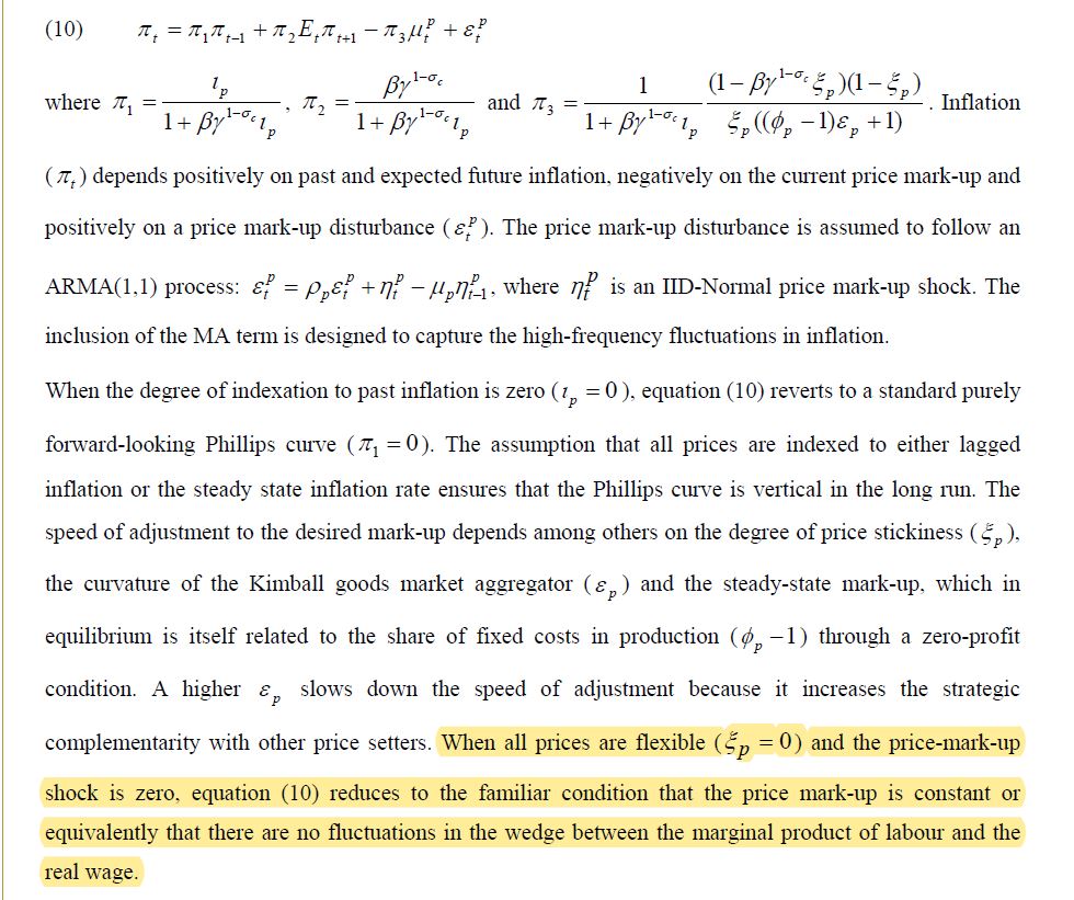
( see figure “inflation”). The highlighted texts mention that " when we set the Calvo parameter to 0, equation (10) reduces to the familiar condition… My question is, would \pi_3 be infinity if divided thoug by 0? Is this the way to derive the inflation for the flexible version of economy?
Besides, if we set Calvo probability to 0, this means firms always get to reset their prices in each period, shouldn’t we also set indexation to past inflation \iota_p to 0 as well? As partial indexaiton only can be present when firms have to stick to their past prices.
what’s the difference between New Classical model and Real Business cycle models. I suppose they all refer to flexible price and wage setting?
Indeed, the main text states that the labor packer uses a Kimball aggregator, while the appendix uses Dixit-Stiglitz. @Max1 do you know anything about this?
I don’t understand your point. The Euler equation is about the consumption choice, not the direct effect on utility. You can hate working, but still want to consume more if you work more.
This is the household utility function where (\sigma_c-1)>0 as the estimation of \sigma_c>1. Hence this implies households would enjoy working, which is the opposite to the assumptions of most models where households enjoy leisure ( thus hate working). I am asking if is unreasonable ?
If we want to assume a hybrid model where parts of the economy (some sectors) enjoys sticky prices and wages, and other parts ( some other sectors) enjoy flexible prices and wages. How to derive the hybrid inflation rate?
If we assume flexible price and wage settings plus one-period information lag for household in receiving macro information. Would be this called " the New Classical version of the SW model"?
The Kimball aggregator is more general and encompasses the Dixit-Stiglitz aggregator. Hence, SW rely on a special case of the Kimball aggregator in the appendix.
If we assume an economy where parts of its final goods are sold in imperfectly competitive markets (price rigidity), while the rest are sold in competitive markets (price flexibility). Then how should we solve the hybrid inflation rate? for example, a weighted average of inflation from both types of markets?
In that case, you need to define which price index you want to consider for inflation. But that should be straightforward. There will be a relevant numeraire in your economy and all prices will be expressed relative to it
What if the inflation for the imperfectly competitive market (price rigidity) part is defined the same way as before (we will end up with the SAME equation as in the Dynare code). Then how am I supposed to solve the inflation for the competitive market (price flexibility) ?
Another question regarding the BGG financial accelerator paper is:
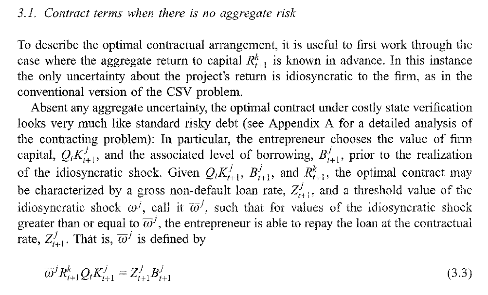
If each entrepreneur’s production is subject to an idiosyncratic shock that affects the return to capital as in Eq(3.3)
Do you mean one version of the model where the Calvo parameter is strictly positive and a second frictionless version where the Calvo parameter is zero?
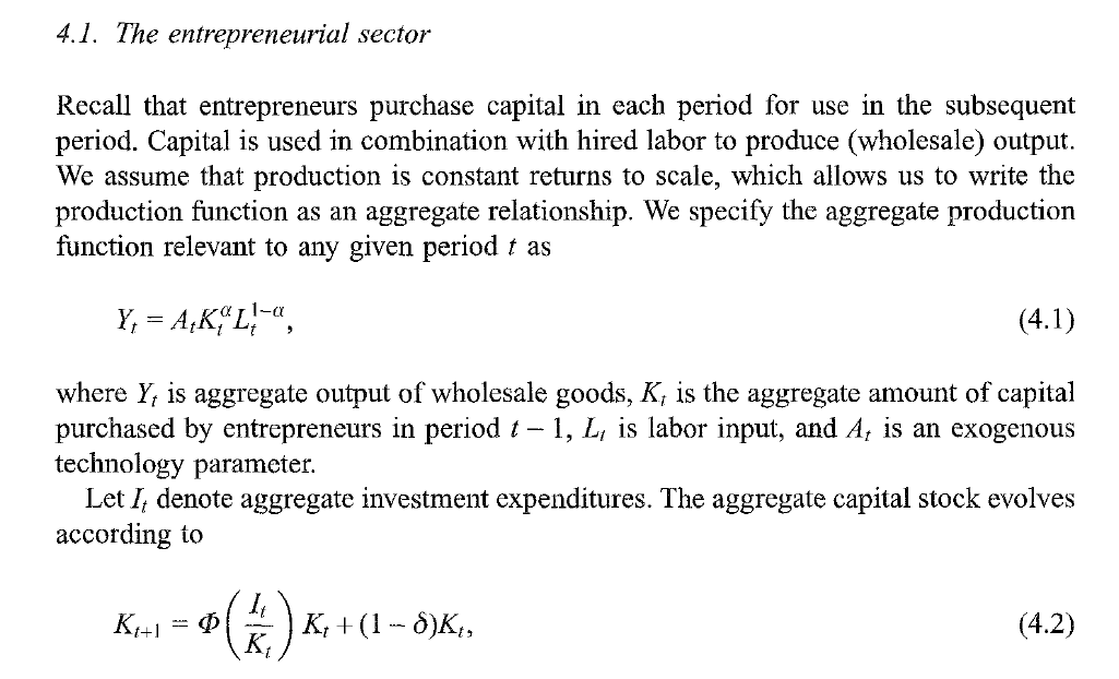
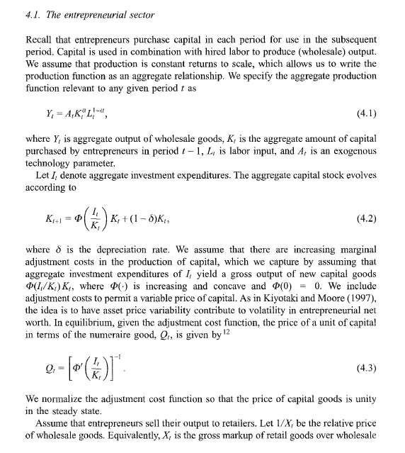
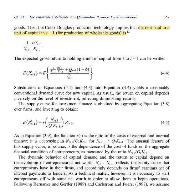
for the entrepreneural sector, it says ( highlighted parts in the second screenshotp) the Cobb-Douglas production technology implies that the rent paid to a unit of capital in t+1 is…
My quesition is, if the entrepreneurs purchase capital rather than rent the capital, then how could the term “rent” apply here??
It does not matter who is the owner of the capital stock. Due to opportunity costs the term “rent” can be applied even if the firm is the owner of the capital stock. In equilibrium, the firm could rent capital to another firm and charge the corresponding fee \frac{1}{X_{t+1}}\frac{\alpha Y_{t+1}}{K_{t+1}}.
Since SW (2007) consider labor augmenting technology growth, but the total time endowment is constant and there is no population growth, the momentary utility function has to fulfill specific restrictions in order to allow for a BGP. According to King et al. (1988) in the case of a multiplicatively separable utility function with \sigma_c>1 the utility part for hours worked must be increasing and convex (as in SW).
Unfortunately, the technical appendix of King et al. (1988) is not available for me.
Can anyone provide me more insights into this type of utility functions that allow for balanced growth but look very counterintuitive on a first glance?
The restrictions of KPR only apply to utility functions before detrending.
You can always cook up a BGP-consistent utilty function by putting a trend variable in there. Take Mertens/Ravn (2011) Understanding the aggregate effects of anticipated and unanticipated tax policy shocks. They have a utility function that is additively separable but without consumption being in logs. To get a BGP, the labor disutility is multiplied with the trend z raised to the appropriate power: c^{1-\sigma}-z^{1-\sigma}n^{1+\kappa}
That solves the issue, but was not envisioned in KPR.
Hi @Julie,
if I’m not wrong, by deriving the marginal utility of labor you can see that utility is actually decreasing in hours worked, at least in steady state.
So, whatever \sigma_c, utility is always decreasing in labor. I guess it is misleading to simply look at the utility function, exactly because preferences are non-separable and the coefficient \sigma_c affects both labor and consumption.
(I realize this reply comes months later, but I hope it’s still useful!)