Dear all,
I recently read the Financial Accelerator in an estimated New Keynesian model by Christensen and Dib (2008). I’d like to repeat the basic model, but it’s a bit unclear that the steady-state calculation is the same for different accelerator factors when the accelerator factor equals zero. I’m not sure if I did the right thing.
Another question is why my figure is not hump type.Each formula is expressed in the form of logarithmic linearization in the appendix of the article.And there is also capital adjustment cost.why my figure is not hump?
Can anyone help me? I will be very grateful.
Have you checked the equations in the original paper for correctness. I remember that at least one equation had to be entered with a different timing structure.
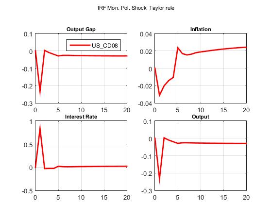
jpfeifer, When running the MMB database of US_CD08 , I can get humped IRFS(like attachments picture).
But when I rewrite US_CD08 without changing any parameters and variables, why do I have to produce a hump-shaped IRFS?The attachment is code I rewrote. There should be no mistake. CD08.mod (2.3 KB)
@aibenaimer1 Please do not ask twice the same question in different threads (I removed one of your posts). Your question here seems also related to (again another thread) the response I have just given here:
In the figure you are showing here, the initial condition (ie the steady state) is the first point of the IRF, this is not the Dynare convention.
Stéphane, thank you for your reply. The picture is produced When running the MMB database of US_CD08, and It’s like the graphics in the paper ‘The financial accelerator in an estimated New Keynesian model’.
My question is when I want to try to repeat US_CD08 code in separate code, why don’t I have similar IRFs?I didn’t change any parameters and variables.I am really puzzled.
I am not familiar with this database of models… You should ask to the guys developing this project, they also have a forum here. If you do not find the same results when using the mod file they distribute, it may be an issue on their side, and as I do not know what they do…
Sorry, I misunderstood your problem here. Did you check if the eigenvalues (a returned by the check command) are the same? I suppose they are not… The most obvious reason being that you must not have the same model. It is difficult to compare both mod files because you are not using the same notations. If I were in your position I would first rewrite the mod file with the same notations.
Without understanding the details, I can see an obvious difference. Your production function is slightly different. If I compare your third equation (for yh) and the fifth equation in US_CD08.mod (for y) I can infer that the productivity does not affect production the same way in both models. In the original mod file productivity is with hours under the power 1-\alpha while in your model productivity appears before the Cobb-Douglas (as would a Hicks neutral trend). This difference is obvious, but I suspect you may have more differences.
Also if you look into the Macroeconomic Model Data Base codes (here lines 13-16) you will see that they append the initial condition (steady state) to the IRFs. So the timing convention is different than the one we have in Dynare figures (which explains the initial jumps).
Stéphane, thank you for answering my question in such a detail. However, I did not change any notation in US_CD08.mod to CD08.mod which was made by me . I just deleted some unrelated code like ‘ Flexible price case’ in US_CD08.mod,in order to make the dynare code run independently. The notations, steady state value,parameters and variables have not been changed. I didn’t change anything. Code is CD08.mod In the appendix. CD08.mod (2.3 KB)
// Model: US_CD08
// Created by Jens Kruk
// Last edited: 2010/09/07 by S. Schmidt
// Christensen, Ian and Ali Dib. 2008. “The financial accelerator in an estimated
// New Keynesian model,” Review of Economic Dynamics 11, pp. 155-178.
var lambda c b m e r h w y k a i cost z mu pi q x f n rp;
You mentioned‘ Also if you look into the Macroeconomic Model Data Base codes (here lines 13-16) you will see that they append the initial condition (steady state) to the IRFs.So the timing convention is different than the one we have in Dynare figures (which explains the initial jumps).’ I don’t know if my understanding is correct?Do you mean that even if my code are consistent with the code in MMB, I will not get the same IRFs like the MMB model?
I still want to ask how the IRFs in ‘The financial accelerator in an estimated New Keynesian model’ generated.In other papers references to Christensen and Dib (2008),they did get IRFs similar to Christensen and Dib (2008), and how did they make them?
Thank you very much for answering my doubts in advance .Best wishes.
Sorry I may be lost. I was comparing the file accelerate.mod (attached in the first post of this thread) and US_CD08.mod (available in the model database).
Yes, even if the IRFs are the same, the IRFs plotted by Dynare will look different because Dynare does not put the initial condition (steady state) as a first point. The IRFs returned by the model database from periods 2 to the last one should be identical to the IRFs returned by Dynare from period 1 to the last one.
Stéphane,I’m not sure whether I understand your meaning accurately. I needn’t have to deliberately repeat IRFs in the paper ‘ The financial accelerator in an estimated New Keynesian model ’? ‘Because Dynare does not put the initial condition (steady state) as a first point’,So it is almost impossible for me to repeat the IRFs in the paper of Christensen and Dib (2008). Is my understanding right?
Once again… I do not know anything of this paper (and I will probably never). My point is just a matter of graphical representation. Even if the IRFs are the same (because the models are the same). The plots returned by Dynare are different from the one in in the model database (I do not know for the paper), because they add a point (the first one) for the initial condition. The IRFs can look different even if they are identical.