Dear Professor Pfeifer,
Thank you for reading this post.
I intend to add a new tax(which will be implemented in 4 periods) shock into the model and compare the difference of irfs with or without this new tax. In other post, your suggestion is to set this anticipated deterministic shock as a news shock in a unit root process, just as:
tau=tau(-1) + e_tau(-4);
I did so while the results display NaN in theoretical moments. How should I improve this?
(I sent you the code through message.)
I am also curious about the trajectory of variables (such as output) in the stochastic model before and after the anticipated permanent new tax shock in 4 periods. How should I realize this?
Thank you for your time.
Best regards
The NaN moments are expected due to the unit root. Unconditional second moments do not exist in this case.
Dear Professor Pfeifer,
I use the follow lines in the code (thanks to your code example in the github which helps a lot) and get irf plots as bellow.
code:
initial_condition_states = repmat(oo_.dr.ys,1,M_.maximum_lag);
shock_matrix = zeros(options_.irf,M_.exo_nbr); %create shock matrix with number of time periods in columns
// set news shock
shock_matrix(1+4,strmatch(‘e_tauh’,M_.exo_names,‘exact’)) = 0.02;
y2 = simult_(initial_condition_states,oo_.dr,shock_matrix,1);
y_IRF = y2(:,M_.maximum_lag+1:end)-repmat(oo_.dr.ys,1,options_.irf); %deviation from steady state
figure
subplot(2,2,1)
plot(y_IRF(strmatch(‘GDPU’,M_.endo_names,‘exact’),:)); % use strmatch to select values
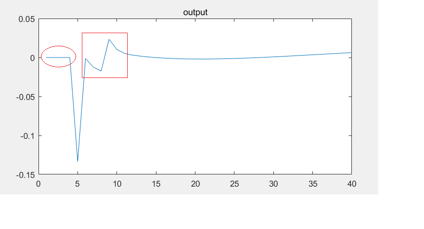
title(‘output’);
irf plot:
I have got a few questions when seeing the plot. Would you please give some guidance?
(1)How should I interpret this kind of fluctuation in the red rectangle?
(2) It seems the permanent new tax shock is unanticipated according to the results as the variables in the model are not impacted between 1-4 periods (as shown in the red circle). I thought the variables might change before the new tax was implemented at t=5 if it’s anticipated. Did I make anything wrong?
(3) I intend to get irf plots with mixed shocks, for example, the model is impacted by a stochastic technology shock at t=0 and meanwhile people know a new tax shock will arrive at t=5. I want to compare the irf plots under technology shock with and without this new tax shock. Does it possible to be realized?
Thank you for your time.
Best regards
Dear Professor Pfeifer,
Thank you so much for your reply.
-
I checked the code but still could not find where the probelm came out.
I think the problem may relate to this new adding tax rate. In benchmark model, the tax rate tauhU is set as a parameter and equal to 0. Then I change it to an endogenous variable and add
tauhU=tauhU(-1) + e_tauh(-4);
into the model. As the code is written in exp() form, tauhU should be exp(tauhU) in the model block. Did I make anything wrong?
-
Please forgive my ignorace. How should I embed stochastic shocks into shock_matrix entries. Would you please give an example?
Thanks again for your precious time.
Best regards
Dear Professor Pfeifer,
Thanks again for your reply.
-
I rechecked the model and find that this new tax variable only shows up in households’ and governement’s bugdet constraint. It seems to be a static variable that only exists at current t period.
Does this mean that people could never anticipate this new tax coming? This seems not in accordance with the economic fact. Is there anyway to improve this?
-
I think you are telling me to change the follwing entry, but I still feel a little confused on how to embed stochastic shocks into this matrix.
shock_matrix(1+4,strmatch(‘e_tauh’,M_.exo_names,‘exact’)) = 0.02;
Taking monetary policy shock e_R as an example, where should I get the values of e_R in these 40 periods? How should I assign shock values into this shock_matrix?
Thank you for your precious time.
Best regards
Dear Professor Pfeifer,
Sorry to bother again.
I’ve got one last question about this:
In AR(1) process e.g. epscU = rhocUU*epscU(-1) + e_c, the steady state of shock variable epscU is generally equal to 1. In case the code is using exp() form, the initial value of epscU is 0.
However, when adding this tax shock equation tauhU = tauhU(-1) + e_tauh(-4), the steady state of tauhU is actually 0 (as I want to see this tax rate varying from 0 to 0.02). Then the initial value of tauhU seems to be -inf in exp() form. How should I deal with this kind of situation?
Thanks again for time.
Best regards
A tax rate is already in percent. So why would you put it in exp()?