Problem with results of welfare analysis

[superj]

Dear Professor Pfeifer,

I mean to analyze the welfare loss under different policies and search for the opitmal policy. I set welfare loss function as in Monetary and macroprudential policies.pdf (823.3 KB)
by Angelini et. al.(2012). However, I don’t understand why the value of output gap and inflation in oo_.var is so small, and also these components in welfare loss function are not in the same order of magnitude. Is there anything I missed in the code? Would you please take a look?(The code is sent through message)

And also, the running of code for searching optimal parameters lasts very long time. Is there any way to shorten the time? e.g. loosen the accuracy of parameter or sth?

Thank you for your time.

[HelloDynare]

@superj

And also, the running of code for searching optimal parameters lasts very long time. Is there any way to shorten the time? e.g. loosen the accuracy of parameter or sth?

At the first time, run the complete Dynare mod file, with your initial guessed parameters.

From the second time, use the following commands to update your parameters and to loop your simulation:

set_param_value(...);
[info, oo_, options_, M_, ] = stoch_simul(M_, options_, oo_, var_list_);

Do not loop the whole Dynare mod file each time. This is strongly discouraged. Also see:

Loop over parameters

You are not actually setting the parameter. What you should do is use the the set_param_value command. Moreover, if you have an analytic steady state, use a steady_state_model block instead of initval. You can find an example for such a loop here: [Need help to check Matlab compatibility). Basically, you need to write a Matlab m-file with the following parts: rhos = 0.8:0.05:1.05; first_time = 1; for i=1:length(rhos) if first_time set_param_value('rho',rhos(i)); dynare your_…

In this way, the whole looping process will be very quick. I met the same issue before. You can trust me

For other parts of your questions, please wait for Prof. Pfeifer’s comprehensive answer.

[HelloDynare]

@superj

However, I don’t understand why the value of output gap and inflation in oo_.var is so small

I’m less experienced in judging the value of variance of output gap, since our definitions or measures of output may be different. But in my project, variance of inflation is indeed small.

Perhaps we can think this phenomenon as follows:
For example, you have the Taylor rule:
\displaystyle\frac{R_t}{R}=\left(\frac{\Pi_t}{\Pi}\right)^{\rho_p}\left(\frac{Y_t}{Y}\right)^{\rho_y}.
And you have the loss function:
\mathbb{L}=\lambda_1Var (\Pi_t) +\lambda_2Var(Y_t).

Now think Var (\Pi_t) and Var(Y_t) as two distortions, externalities, or rigidities that you want to remove. Given predetermined \lambda_1 and \lambda_2 and given varying \rho_p and \rho_y, you could expect your policy tool R_t can correct / remove \mathbb{L}, with some hidden relations between \lambda_1 and \rho_p and between \lambda_2 and \rho_y. Because actually you have a weighted tool R_t of two instruments \Pi_t and Y_t in your hand. It is equivalently to say we have two instruments \Pi_t and Y_t to remove two distortions Var (\Pi_t) and Var(Y_t).

However, if maintaining the previous Taylor rule, we reset the loss function as:
\mathbb{L}=\lambda_1Var (\Pi_t) +\lambda_2Var(GDP_t), by GDP_t\equiv p_{t}Y_t. Then I cannot guarantee Var(GDP_t) has a small value.

All above are my humble opinions. Please wait for Prof. Pfeifer’s correction

---

And I completely have no idea on

@superj

also these components in welfare loss function are not in the same order of magnitude

[superj]

Dear HelloDynare,

Thank you very much for your reply. I actually used csminwel function as in Optimal policy parameters in a non-linear model. I wonder if I could change the options in csminwel to shorten the steps of searching parameters. Do you have any advice?

Thanks again for your kindness.

[HelloDynare]

Sorry, @superj, yes, I viewed the linked topic before. I remember that csminwel is also a local method. For my situation, set_param_value(...) seems to be adequate. So I’m afraid that I fail to give you further suggestion.

Instead, CMAES is a global method. I attempted to apply CMAES in a Ramsey situation. See

Two m files and two mod files

Dynare finds the result more quickly than a two-instrument version of RamseySOE, so we didn’t notice the uniqueness. However, in the two-instrument version, we indeed realized it, very sensitive to our initval guess. So here is my question: Will CMAES be helpful in Ramsey problem? (I plan to substitute CMAES for fminsearch function) Besides, your reply gives me the impression that the upper bound of the welfare of OSR-SOE, by deliberately choosing Taylor parameters, can dominate the lower…

But

@jpfeifer

CMAES will not help. It’s not about your optimizer in the steady state file converging to something only locally optimal. It’s about Dynare’s routines internally converging to a local optimum. As of right now, there is no way to change this other than trying different initial conditions. But even with a global optimizer, that would be someone should do to make sure results are not driven by initial conditions.

---

Cmaes vs csminwel

csminwel is a Newton-type local optimizer. If you are close to the global mode, it will quickly converge to this this mode. But it can also converge to a local mode, i.e. fail to find the global one because it is local. cmaes is a global optimizer. It will be slower but has a higher likelihood of finding the global mode instead of just a local one.

Welcome your ‘‘user experience’’

[jpfeifer]

1. The bottlenecks are you not specifying irf=0, so in each iteration the IRFs are computed and the crazy TolFun set in the steady state file.
2. Welfare losses from business cycles are often small. Two percent output volatility also looks decent.

[superj]

Dear Professor Pfeifer,

In the result of my code, the var of output gap is like 5e-04, and var of inflation is like 5e-05. It seems so small that I have never seen such values in any papers. So I wonder if I miss any details?

And also, I get optimal value of the weight of inflation in Taylor Rule is like 38, which is so much larger than the prior or posterior value (around 1.5). Does this make any sense? And what’s the economic meaning if the weight of output gap in Taylor Rule is a negtive number?

Many thanks for your time on this.

[jpfeifer]

1. It’s more intuitive to look at standard deviations. As I mentioned above, they are in the range of 0.02, i.e. 2 percent per time period in your model. That is normal.
2. Having the weight on inflation feedback going to infinity is not uncommon. This has been discussed in several posts here on the forum. The typical solution is to impose an upper bound.
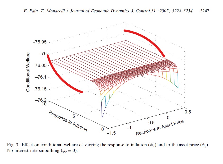
3. With respect to negative output feedback, it is hard to interpret. Is the number meaningful in magnitude? Often times, the objective becomes very flat. If you have an inflation feedback of \approx 40, then having output feedback of -0.5 might not do anything.

[superj]

Dear Professor Pfeifer,

To the 2nd one, I wonder if it’s meaningful to display this big value of weight on inflation feedback in the paper? Is there any papers have done this before?

And also, if the optimal value of this weight on inflation feedback is actually so big, why prior and posterior value is around 1.5? Is it because it’s difficult to achieve such big value in practice? What might be the appropriate upper bound of inflation feedback？

Looking forward to your advice, and thank you for your time on this.

[HelloDynare]

@superj

To the 2nd one, I wonder if it’s meaningful to display this big value of weight on inflation feedback in the paper? Is there any papers have done this before?

@superj

Is it because it’s difficult to achieve such big value in practice? What might be the appropriate upper bound of inflation feedback？

FYI:

Small Variance Value in Ramsey Policy NK Model

Hello, after reviewing your dialogue, I would like to complement just one remark on the following quote: This is not unusual. I read SGU 2006 expanded version. On page 22 footnote 10, they did unconstrained OSR as well, finding a similar pattern: [image] Note the sentence “The associated welfare gain is about one thousandth of one percent…”. I experimented a 3D-diagram of welfare with inputs of \alpha_{\pi} and \alpha_y. The welfare surface is extremely flattened with varying \alpha_{\pi}. …

---

Optimal Simple and Implementable Monetary and Fiscal Rules: Expanded Version

and for example, your searching space is located in the following flattened surface: