I downloaded the dynare code of Iacoviello and Neri(2010) from the homepage (as attached) in order to replicate the results of comparison between model moments and data moments.
I add option “moments_varendo” into estimation command in the dynare code, but found that it displayed errors as the original code setting “mode_compute=4”. Then I tried mode_compute=5 and 6, and found that the posterior means of parameters were not identical to the values in their paper. Meanwhile, all the posterior distribution of theoretical moments which are stored in oo_.PosteriorTheoreticalMoments.dsge.covariance seems much larger than the values showing up in Table 5 of the paper. e.g. the standard deviation of consumption is 1.57 in the table while the sqrt(oo_.PosteriorTheoreticalMoments.dsge.covariance.Median.data_CC.data_CC) is 3.87.
Did I make any mistake in replicating the results?
Looking forward to your reply and sincerely appreciated on you kindness.
Best regards
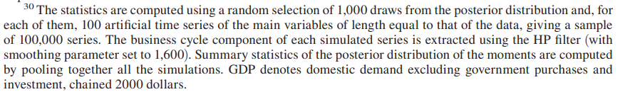
Coincidentally I am after the same thing. Footnote 30 in Iacoviello and Neri(2010) explains how they construct their moments and a very similar question has been asked in this legacy post.
Essentially the first part can be replicated through moments_varendo, as done by James. Johannes, in the legacy post you point out that the second part is not really necessary due to linearity, hence no artificial time series is needed, just the theoretical moments. However, in terms of replicating the moments of the above paper, is it somehow possible to simulate data for the each posterior draw as described by Iacoviello and Neri(2010)?
Although the differences in parameter estimates are not quite sizable, I do not think this could explain the differences of the moments.
Actually I did not compare the moments between model and the data. I just compared the results stored in oo_.PosteriorTheoreticalMoments.dsge.covariance and posterior predictive moments the authors displayed. In case that both are the evaluation about model fit, I consider the results may suppose to be close.
When calculating the posterior predictive moments, the authors used HP filter on the simulated series. Does this influence the results of comparison above? But how should I get “HP filtered” results of “moments_varendo” ?
I tried adding a variable defining first-difference filter(different from HP filter though) e.g. dc=c-c(-1), and found it’s closer to the value in their paper. So I think it may be the filter thing.
What happens if you take the posterior mean and run stoch_simul with the hp_filter option. Is that close? In that case, it might be the missing HP-filter.
With an additional question:
If I want to calculate the posterior predictive moments exactly as they do ( they randomly select 1000 draws and for every draw they simulate 100 time series of the same length equal to the data), taking standard deviation as an example, there are two cases:
one is to calculate the medians and quantiles of standard deviation for artificial time series under each draw and then calculate the mean of them for all 1000 draws;
the other is to calculate the means of standard deviation for artificial time series under each draw and then calculate the median and quantile of them for all 1000 draws.
Which one should be the right case ?
I have searched the forum before and learned your posterior_function_demo (many thanks to your code). Now I have read out the simulations of 1000draws * 100series * 60periods as I request and want to calculate the moments.
I’m a little confused about the order of calculation. Which way bellow should be the right case ?
(1) to calculate the medians and quantiles of standard deviation for artificial time series under each draw and then calculate the mean of them for all 1000 draws;
(2) to calculate the means of standard deviation for artificial time series under each draw and then calculate the median and quantile of them under all 1000 draws.
That’s hard to tell. My reading is that you compute the standard deviation for all all 1000*100 series (the 100000 series the paper mentions) and then calculate the quantiles.
Is it possible to run the posterior_function in a fully separate step after the estimation has finished? In other words, the mod file does not explicitly contain the posterior_function command and hence the function is called from a separate m file after dynare has finished the estimation. I’m not sure if this is possible because the posterior_function requires the current parameter draws (i.e xparam1).
Does the 100 time series mean M_.endo_nbr=100, which can be obtained from ys in the posterior_function_demo
Inside the posterior_function_demo I am using output_cell{1,1}=oo_.var, which gives me later the variance-covariance matrix for each draw of my observables specified in var_list. From there I compute the mean standard deviation (for the 1000 draws) and compare them to the data counterparts. Is that correct? Also, is this the same approach as the authors describe above?
From what I read above, not completely. oo_.var will store the variance for one time series and one draw. You still need the additional step of 100 time series for each draw.
Thanks for your help Johannes! I have changed now the posterior_function_demo such that it produces 100 time series each for draw. I request the following three things inside the m file:
output_cell{1,1}=oo_.var;
output_cell{1,2}=ys’;
output_cell{1,3}=simulated_series_filtered;
However, I seem to have done something regarding how the data are stored in oo_ structure.
Weirdly when I call posterior_function_demo inside the mod file with the simulated_series_filtered definition, Matlab gives me a warning that it can’t save the oo_ structure because it exceeds the 2GB limit.
When I call posterior the function from a separate file (i.e. running posterior_function_demo outside the mod file) and I type into the Matlab command box oo_.posterior_function_results I see the entire output (it’s a 1000 x 3 array). However, when I now load the (last) result mat file, it overwrites the current oo_ structure and it “deletes” the output_cell{1,3}=simulated_series_filtered. I thought it would just add to the old oo_ structure.
So I am wondering whether have I made a mistake when I added the simul_replic=100 to the posterior_function_demo file? I have attached the adjusted file below:
I would need to see the files. But a few general remarks.
You are requesting 12 endogenous variables with 136 periods and 100 replications for 1000 draws. That will of course result in a very large object that requires a lot of storage. But you can save that file manually using save('myFile.mat', 'Variablename', '-v7.3')
You cannot easily run posterior_function_demo outside of the mod-file, because Dynare runs this file within a loop.