Dear Johannes,
My work is based on the non-stationarity of hours worked. I compare the IRs from the actual and the simulated data.
The actual data tells me that hours worked are non-stationary. What I did in my work is following:
- I estimate hours and GDP using Structural VAR with long run restriction. In VAR model: first variable is hours and second variable is GDP. Also, first shock is labor supply shock and second shock is technology shock. So, the interpretation will be : only a labor supply shock has a permanent effect on hours and both shocks will have a permanent effect on GDP.
- Then, I build a DSGE model to obtain the non-stationary hours (simulated data) and apply the SVAR procedure that I explain in above. I adopt the DSGE model proposed by Chang et.al (2006) including permanent labor supply shock which yields non-stationary hours. I also have a technology shock. Both shocks have a unit root process. So, this model implies that both technology shocks and labor supply shocks have a permanent effect on GDP; that only labor supply shocks have a permanent effect on hours worked.
I got some feedback in my presentation saying 1. I cannot use the preferences that I have (please see dropbox.com/s/xn4g6ywicjv1i … 8.png?dl=0 ).
2. The long run restriction is not valid unless I convince people that the reason why hours are non-stationary in the data is due to labor supply shock.
It is still not clear to me which types of preferences I should you? Where should I look? i would greatly appreciate if you could give me some suggestions about it.
Best
Hi,
I don’t really see what the problem is. Due to log consumption, your preferences imply a balanced growth path in the absence of permanent labor supply shocks. So what is the objection?
Regarding identification: your model and the data are consistent in that the model satisfies the identification restrictions you apply to the data. So I don’t see a problem here. Of course, we don’t know the data generating process so one might come up with alternative stories explaining non-stationary hours. But without outside evidence, your story is as good as any other (and in the tradition of using preference shocks as a stand-in for more structural shocks a useful first step)
Quick sidenote: be careful with “non-stationarity”. It just tells you the data is not covariance stationary. But there are many reasons, for example structural breaks. You seem to have one particular form of non-stationarity in mind: a unit root, i.e. hours are I(1). To establish this, you may need a test that allows you to actually reject that the data has no unit root. That is, a Dickey-Fuller test is not sufficient, rather you need a KPSS-test to make a convincing point
Thank you very much. I totally agree the points you mentioned.
Their point is that: VAR and model specification are the same but it comes from an assumption of the model. Imposing that restriction is not guaranteed in the sense that is an assumption of the model. They asked me what if the specification of preferences is incorrect?
Maybe I need to re-frame my paper and say that I am looking at whether labor supply shocks have a long run effect on hours worked.
Normally, I start my presentation showing some figures and telling that hours are non-stationary. Thats why hours need to enter into VAR in first difference. Then, telling my VAR restriction and presenting the model.
Any other suggestions will be greatly appreciated.
Best
I see. Justifying the preference shock as structural may be hard. As you said, convincing your audience may be a matter of a different framing. You could for example interpret your exercise more like a business cycle accounting (Chari/Kehoe/McGrattan (2008)) exercise where future research needs to determine the actual microfoundation
I have a question related to stationarity. Should the variables used for estimation pass statistical stationarity tests?
From your paper, ‘A Guide to Specifying Observation Equations for the Estimation of DSGE Models’, I understand the variables must be non-trending/stationary.
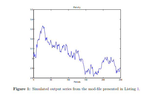
I have US data on inflation and interest rates from 1959 to 2009. They are non-trending but they fail KPSS and ADF tests for stationarity in levels. And figure 1 from the paper (simulated output) seems to have a trend over long periods. It looks like the decline in the inflation rate and interest (US data) since 1980s…and may fail stationarity tests.
Can we conclude that stationarity is assumed in the model? That is, even though it fails statistical stationarity tests, we assume that these variables (inflation and interest rate) are stationary. Is it also why inflation and interest rates are used in VAR-type models in their levels even when they fail statistical stationarity tests? Kinda confusing, right? Like on what basis can we say a variable is stationary…visual inspection? statistical tests? I am trying to understand these issues.
This is tricky. First of all, most theoretical model tell you that the data is stationary. The big question is whether the empirical data satisfy that requirement. Most people tend to say yes for many countries and therefore do not rely on formal statistical tests. After all, we all know the problems with low power of tests in short data and problems like structural breaks etc. There is also the problem of near unit-root behavior. The latter is regularly assumed to be the reason of the persistence in inflation, i.e. the central bank having a slow-moving inflation target.
Regarding VARs, there is the Sims/Stock/Watson result. See Is the effective federal funds rate stationary? - #2 by jpfeifer
1 Like