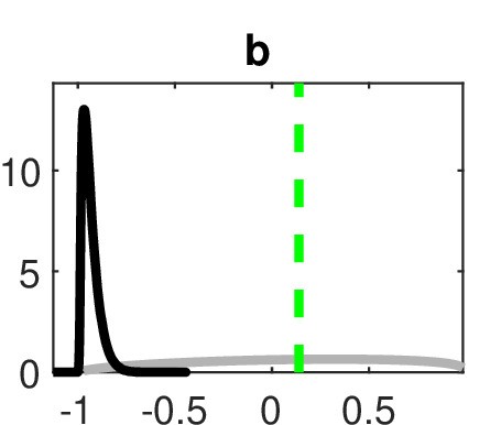
I’m getting a strange (to me) result. I estimate the mode (using mode_compute=5, though I’ve tried others), and for the habit-formation parameter, b, I get b=0.139, which is small but reasonable. When I do full Bayesian estimation with mode_compute=6, the posterior mean is -0.936, near the lower bound of the support for the prior (beta distribution on [-0.99, 0.99]), and the mode is far from the entire posterior distribution, as you can see here.
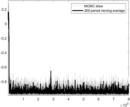
I thought it might be a convergence issue, but I increased the number of replications, different mh_drop settings, etc. but get the same result. This is the trace plot.
I will note that there’s another parameter in the model that is supposed to be non-negative, but comes out at around -0.02 (both the mode and mean). When I set it equal to zero and reestimate, b comes out with a mode and mean around 0.2. So I will probably go with that result, but I still find the result when I estimate both parameters puzzling.
Thanks for the quick response. To clarify, the other parameter, \kappa is the coefficient on quadratic investment adjustment costs. I think it has to be non-negative, but it’s possible there’s a well-defined solution with \kappa<0, as it’s a large model with other adjustment costs.
Do you mean when I set \kappa=0? I get a lower posterior density.
I was getting a non-positive definite Hessian finding the mode if I used a prior with a lower bound of zero but that had positive density at zero.The mode_check diagram for that parameter was still rising as the value went to zero. If I use something like a gamma distribution with density zero at \kappa=0 then I get a positive posterior mean for b, but that forces the posterior mean of \kappa to be positive.
With the prior I used, I thought I would get an estimate of \kappa that had a 90% HPD interval that included zero, and a reasonable posterior mean for b (like the b=0.14 at the mode), but in fact the HPD for \kappa was [-.034,-0.020], centered right on the mode, while I got the extreme posterior for b so far from the mode. I could have chosen a prior for b with [0,1] support, but b<0 is feasible, so a small negative posterior mean for b would have been fine, but not b=-0.94.
No, I meant if you plot a trace plot of the posterior, what happens?
I still stand by the point that the lower bound must be 0. What you describe sounds like a case where the prior distribution is ill-defined. \kappa<0 would mean that changing capital would increase capital.
I’ve attached a trace plot of the posterior. traceplot_nmusd4_posteriordensity.pdf (157.7 KB)
I think what’s going on is that there must be two modes for b. If I use a prior for b with a mean of 0.1 I find a mode of around 0.2, but with a prior mean of -0.8 I find a mode of -0.94 with a higher likelihood.
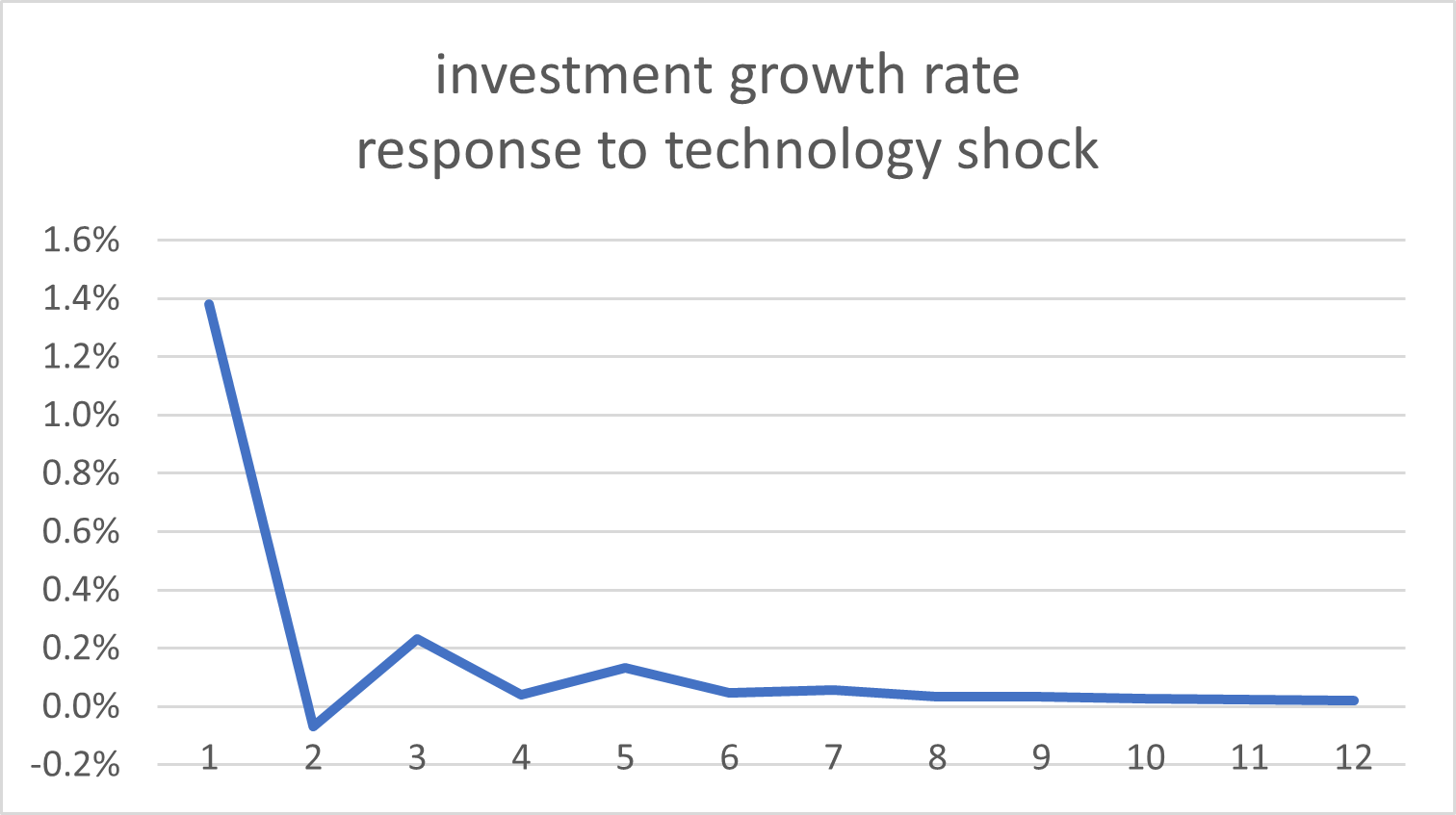
The model has other features, like capital adjustment costs, that may make \kappa<0 feasible, though maybe implausible.If it were infeasible, wouldn’t it blow up the irfs? This is the irf I get for the growth rate of investment with \kappa=-0.027:
The big picture here is that I’m comparing two models, call them A and B, hoping B knocks out A. If I estimate model A I get \kappa\approx 1 and b\approx 0.4. Model B assumes \kappa=b=0 and gets a much higher log data density (model_comparison gives Model B probability \approx 1). Then I estimated Model A U B, hoping to get \kappa=b=0, but instead getting \kappa<0 and b<0 (at least in the 90% HPD interval). This isn’t a Dynare question, but I’m trying to figure out what that implies.
I am not sure I get the point. The mode is for the posterior. Of course the mode will change if you change the prior.
No, they would not blow up. But I would still argue that economically, \kappa needs to be restricted to positive values. I am not aware of any paper allowing negative values. After all, that is also the reason for using quadratic costs.
Sorry, I was unclear. I had in mind the original question of how mode_compute=5 could find a posterior mode that was so far from the posterior mean with mode_compute=6. This is with the same prior. My conjecture is that the posterior density is bimodal, and mode_compute=5 found a local maximum, as I presume it just looks for the nearest upward path. Am I thinking about this incorrectly?
Ok, let’s suppose \kappa<0 is infeasible. This is probably getting too far into methodology/philosophy, but your question was “why have a prior that includes that in the support?”. Maybe this is a non-Bayesian way of thinking, but I want it to be possible for the model to fail (versus an alternative model), meaning to find that \kappa = 0 (i.e. that 0 is in the 90% HPD interval). That’s not possible if the support of the prior is only on \left[0,\infty \right) . I think of the support on the infeasible range as allowing for probability the model is wrong rather than forcing it to be correct.
Again, I’ve estimated a model (B) that assumes \kappa=0. Now I’m estimating a larger model B U A in which \kappa>0. I want it to be possible to conclude that model B U A is no better (or maybe worse) than model B by itself, because \kappa is likely zero (or worse, negative). I don’t think it’s possible if I restrict \kappa to be positive.
Incidentally, I have done model_compare with B vs A, and B has a posterior probability of 0.9999. But since they’re not mutually exclusive, I wanted to consider B U A.
Yes, you can clearly see in the trace plots that the MCMC moves to a higher mode. That is, unfortunately, not uncommon.
This indeed is a non-Bayesian way of thinking about the problem. Models rarely “fail” but are just unlikely to be the data generating process. A posterior probability of 0.9999 means model B is 10,000 times more likely than model A. That should be sufficient.