I have a three variables deterministic non-linear model with three steady states. Two of them are saddles and the other one is unstable (with complex conjugates) and located between the two saddles. The model has one state variable.
I want to know whether this model admits multiple equilibrium paths (global indeterminacy). Specifically, whether there is a common initial condition around the unstable steady state such that the economy can converge to one or the other (saddle) steady state.
To be sure if this this possible I have to numerically compute the common initial conditions (if they exist).
I wonder if this can be done in Dynare using a sort of “reverse” shooting algorithm using the perfect_foresight_solver() or simul() commands.
The conjectured algorithm would be the following (please correct me) :
For steady state 1 (a saddle), set the corresponding steady state value as an end point using “histval” and set the initial value for the state variable arbitrarily. Use perfect_foresight_solver() or simul() to find the path converging to this steady state.
Repeat step 1 for a grid of initial values around the steady state value of the state variable associated with the unstable steady state.
Repeat step 1 and 2 for steady state 2 (the other saddle).
Compare the grids and compute the range of common values.
Would this work with Dynare? Should “histval” be exactly the steady or somewhere close to it?
Your algorithm sounds correct, but I would forgo using blocks for directly setting oo_.endo_simul to the desired values before calling perfect_foresight_solver. See e.g. Loop in perfect foresight context
Yes, you need to set the exact steady state as the terminal condition.
I followed you advice, but I would like to double check a few things related with perfect_foresight_solver. This is my exercise (for one of the steady states):
I compute the steady state with an external file.
My mod file contains the endval block, and corroborates the steady state solution using the resid, steady, check, and model_diagnostics options.
I use perfect_foresight_setup in the mod file to define oo_.endo_simul.
oo_.endo_simul is then a matrix with first column of zeros and the rest of the columns with the steady state values.
Then, I loop for diferent initial values of the state variable (the only state in this model and with one lag) by replacing the corresponding cell in the first column of oo_.endo_simul and running perfect_foresight_solver.
I store the simulations where the solver works ( oo_.deterministic_simulation.status == 1 ).
My doubts are:
a. The solver fails in most of the cases with the default option, and then uses homothopy, where it works. Should that sign a red flag on the results? (The difference between the penultimate and the last column is below 1e-06).
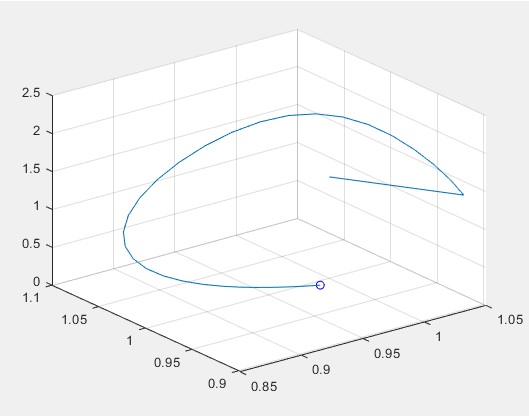
b. When it solves, the solver updates the zeros in the first column of oo_.endo_simul. However, there is a “big” step between the values in column one and column two. Thereafter the steps are small until convergence (See figure*). What is the solver doing for the first column? Should I consider this column for plotting the transition given the state variable is lagged?
Thank you!
*figure: 3-d. x,y axes are the control variables, z is the state. Blue circle is the steady state. Straigt line is from column one to two. Curve from there is column two to end.
I am not entirely sure I can follow your approach. Dynare switching to homotopy is common and typically no reason to worry. What you report with the first entry is worth investigating a bit deeper. The very for column stores the initial condition, which is updated in steps by homotopy. The only thing we care about from the first column are the state values. Everything else is arbitrary.
Thank you for your reply. I checked what you mentioned:
My approach is basically to have an idea about the global dynamics in a model with 3 stedy states by numerically exploring the parameter space using the perfect_foresight_solver with different initial values for the state variable.
Regarding the first column in oo_.endo_simul, you are right. When the solver finds a solution this column only contains the initial value for the state variable, i.e, it remains exactly as set before perfect_foresight_solver (what I described in b) of my second post is actually when the solver does not find a solution, so my bad!).
Where I can find a detailed treatment of the homotopy approach in Dynare? I have only found descriptions about “solving the full problem with a smaller shock and then using this solution as the starting point for the next, bigger step”, but my case is a perfect foresight transition dynamic problem (no shocks) and I would like to know better what Dynare is doing with this option.
which shows that instead of immediately trying to jump from the initial to the terminal condition, you attempt a smaller jump based on weighted average. When that works, you increase the size of that jump based on the last successful iteration.