Hello!
I have a question regarding the paper (Sims, 2021) https://sites.nd.edu/esims/files/2023/05/financial_constraint_2017.pdf, specifically about the case when a collateral constraint applies to intertemporal debt.
I am struggling to understand how to solve this model using OccBin, because the activation of the borrowing constraint depends on a stochastic borrowing limit.
In particular:
- When \xi < \delta , we have \mu > 0, and the borrowing constraint becomes binding.
- When \xi > \delta , then \mu < 0 , and the constraint becomes non-binding.
The difficulty is that the activation of the constraint depends on the value of \xi , which is an exogenous parameter that we specify manually in the code.
Thus, I am not sure how to properly implement this condition in OccBin, since constraint activation is not purely endogenous to the model’s state variables but depends directly on \xi .
I am not sure I understand the point. \xi_t is an exogenous variable that follows an AR-process in that PDF. Of course it can enter the borrowing constraint like any other variable.
Professor @jpfeifer, I’m having trouble formulating the correct condition for OccBin in this context. What I mean is that, in solving this system, the steady state is determined through the expression μ = δ/ξ − 1. If I impose a constraint like min(mup, exp(k) * u_constr * q_K - exp(I)) = 0, then for ξ > δ, we get μ < 0. In that case, the steady state cannot be found, because the minimum becomes negative rather than positive.
I don’t follow. What is the baseline regime, i.e., where is the steady state? When the constraint is binding or not binding. That will determine how you need to implement it in OccBin. The baseline regime must be the one with the steady state.
In this context, when ξ < δ, the constraint becomes binding, and the system can be solved. I was trying to implement the solution similarly to the standard OccBin example, where we solve for b = M * y (e.g., with M = 2). In that setup, we can specify a constraint like:
[name='constraint', relax='borrcon']
b = M * y;

[name='constraint', bind='borrcon']
llambda_b = 0;

occbin_constraints;
name 'borrcon'; bind llambda_b < 0; relax b > M * y; end;
Or, in the perfect foresight setup, it would look like:
min(llambda_b, 2 * y - b) = 0;
Is it possible to implement the borrowing constraint in this model using OccBin in a way similar to the standard OccBin example?
I want to implement it this way because I’m interested in seeing whether the constraint becomes binding or not in response to an unexpected shock. However, it seems that by setting the value of ξ exogenously from the start, we are effectively pre-determining whether the constraint will be binding or not.
Professor @jpfeifer, thank you very much! I now understand how to proceed, but I have a question:
How should the OccBin constraint be specified when the model’s main code and the steady state computation are located in separate files?
I haven’t been able to figure out how to correctly include a block like:
occbin_constraints;
  name 'borrcon';
  bind mup < 0;
  relax b_1 > 2*y_1;
end;
When I insert this type of constraint directly into the .mod file, I get the following error: Unrecognized function or variable ‘occbin_borrcon_bind’.
I would need to see the files.
But where is the steady state file?
Now the param_core.m is missing.
At the beginning of the steady state file, you need
%initialize constraint parameter for passing through
occbin_borrcon_bind=M_.params(strcmp('occbin_borrcon_bind',M_.param_names));
main_steadystate.m (3.0 KB)
Professor, thank you very much for your help! May I ask one more question?
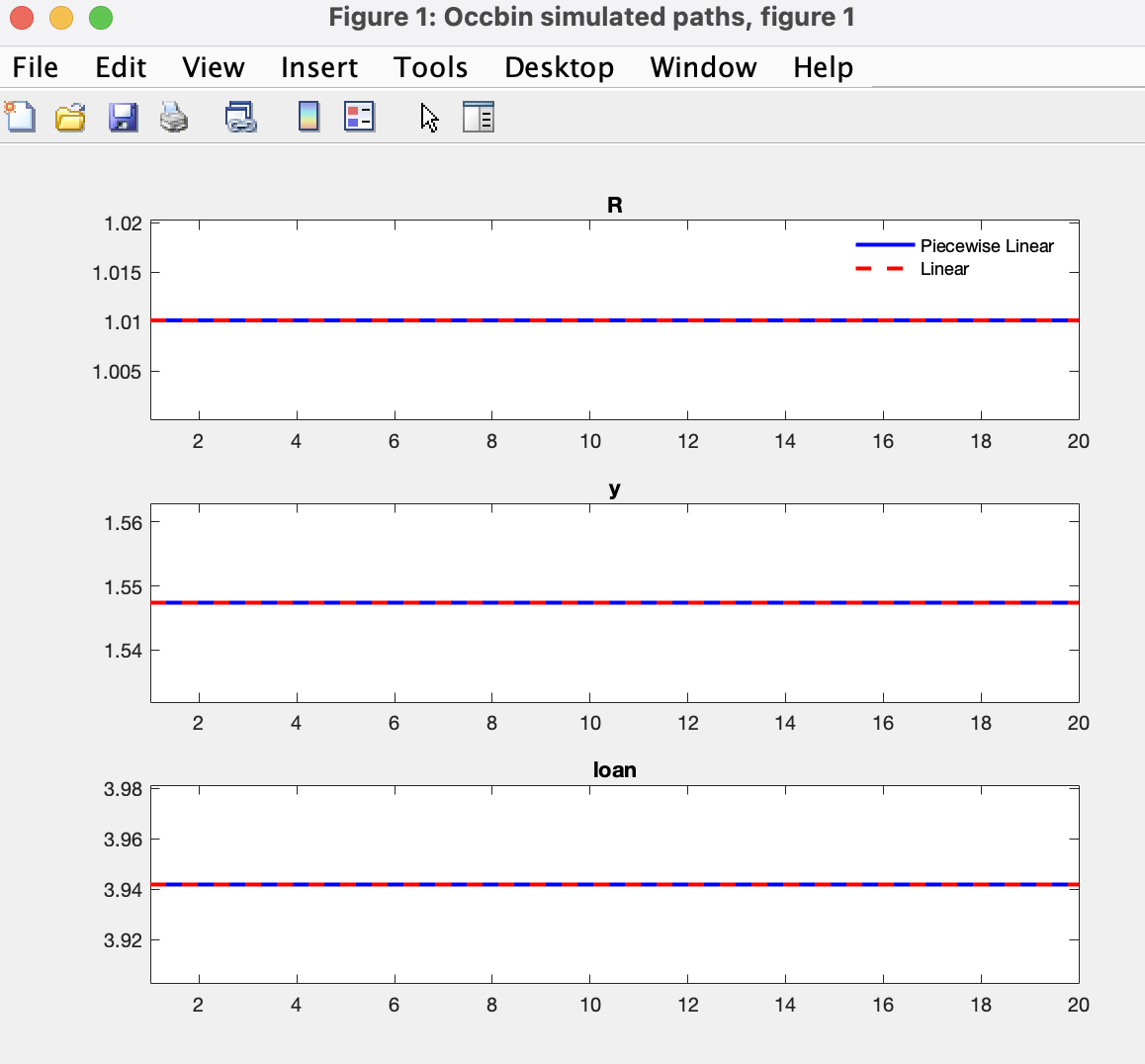
I just want to clarify whether I’m setting this constraint correctly, as the resulting graphs seem odd – they show no dynamics at all. Moreover, the trajectories for both the piecewise linear and linear cases are identical, regardless of the size of the shock I apply.
Run
occbin_graph y R loan z_cb pi;
to see that for some reason only pi moves. That is indeed unusual.
When I apply a larger shock, the variables do show dynamics, but the piecewise linear and linear trajectories still coincide.
That usually indicates that the constraint does not become binding.
I suspect this issue arises because my capital accumulation equation is specified at time t, which means the constraint should involve k(-1). However, OCCBIN does not support lagged variables. When I rewrite the capital accumulation equation in terms of t+1, I encounter a Blanchard-Kahn error.
You can always define k_lag=k(-1) and use k_lag in the constraint.
Thank you, Professor, for your help! I’ll continue investigating to figure out what’s going wrong.