Hi
I have a fledgling question. I apologize for this low level question. If in the initial setting the number of equations was less than the number of variables, can the same number of shocks be added to equalize their number? For example, the number of equations is 33 and the number of variables is 36. Now define three shocks for the three selected variables. Does this cause problems in the results or not?
For example, you have a Taylor-type monetary policy rule. This is one equation. Then you annex a monetary policy shock exp(em) at the end of this rule. But it is still one equation, not two. Alternatively, we say AR(1) forms are equations, pure eA, eZ, em innovations are shocks.
But you can make 3 variables to be 3 AR(1) equations, ended with 3 new shocks. I think this is feasible.
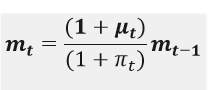
Many thanks for your reply. Your answer is understandable for the example you gave of Taylor-type monetary policy. But suppose, for example, that my monetary policy is not Taylor-type, but as follows. M(t)=(1+mu(t))*M(t-1).
Here, at first glance, I consider (mu) as unknown. But this makes the number of my equations less than my unknowns.Do I have to define monetary policy shock here(AR(1) for mu) ? It is not necessary to define this shock for my results(For example, I just want to look at the results of the technology shock) , but it seems that I have to define it for the equality of equations and unknowns.
If I were you, then
Case 1: \mu is time invariant, then you calibrate or estimate the value of \mu. Make \mu known.
Case 2: \mu_t itself as a pure shock, following \mathcal{N}(0, \sigma_{\mu}). So your endogenous variable number -1, 
Case 3: \mu_t is an exogenous AR(1). It is possible, because the money growth is not as stable as expected. I saw some papers have a few shocks, and they leave most IRFs into the appendix, without further explanation.
Case 4: \mu_t is an endogenous AR(1), for example, \mu_t is a recursive function of \mu_{t-1}, debt \frac{D_t}{D_{ss}} and/or interest rate \frac{R_t}{R_{ss}}, but their relative weights, say \rho_{\mu}, \rho_{d}, \rho_{r}, are to be determined, then we go back to Case 1 
Then you can compare Case 1- 4, according to some criteria. Wow 
You may request the help of Prof. Pfeifer. I’m new in macro.
The issue is that you need exactly as many equations as endogenous variables. Otherwise, there is no way to uniquely determine their values. Adding shocks, i.e. exogenous variables does not help.
Dear Professor jpfeifer
Thank you very much for your response. I meant to add a AR(1) Equation to the equations here. For example, the monetary policy rule is as follows : M(t)=(1+mu(t))*M(t-1)
I know I have to write an equation for any endogenous variable. I look at the equations and see that I do not find any equation for the mu. So I define it as AR(1):
mu=rho_mu*mu(-1)+epslon_mu
Now I have one more equation (Because this AR(1) is written in the model block) and the number of equations and unknowns is equal. However, I do not seek to analyze the results of the money growth shock (epsilon_mu).
So when I wanted to see the effects of a shock (For example, technology shock), I might inadvertently have multiple AR (1) and shocks. So the choice of the number of shocks is not entirely up to us
I still don’t get it. If money grows over time in that equation, no steady state will exist. If you are not interest in a time-varying mu, then simply drop it, i.e. set it to 0.
I think this will solve the problem:
so mu_ss=pi_ss
Of course, I just mentioned this as an example.
No, adding shocks for the sake of it won’t solve the problem.
If as in your example, you have 36 variables and 33 equations and then add 3 shocks, then you end up with 39 variables and 36 equations (the previous 33 + the AR processes for the new shocks).
You need to dig into your initial model to see what equations you are ignoring or whether you have variables that are redundant or are already determined (solved for) so that you can end up with a system of 33 equations and 33 variables.