//------------------------------------------------------------------------------
// RANK_gaps_clean.mod
// (all variables are log‐deviations from their steady‐state = 0).
//------------------------------------------------------------------------------
var pi // π_t: price‐inflation gap
y_gap // ŷ_t: output (and consumption) gap
w_gap // ω̃_t: real‐wage gap
n_gap // ñ_t: employment (hours) gap
d_gap // d̃_t: profit gap
pi_w // π^w_t: wage‐inflation gap
c_gap // c̃_t: consumption gap (= y_gap by goods‐market clearing)
i // i_t: nominal interest‐rate gap
nu // ν_t: monetary‐policy shock (AR(1))
r_gap // r^gap_t: real‐interest‐rate gap = i_t − E_t[π_{t+1}]
mu_w; // μ^w_t: wage‐wedge = w_gap − (φ·n_gap + c_gap)
varexo eps_nu; // ε_{ν,t}: monetary‐policy innovation
//--------------------------------------------------------------------
// 1) PARAMETERS & COMPOSITES (all steady‐states = 0 in gap form)
//--------------------------------------------------------------------
parameters
beta // discount factor
sigma // inverse EIS = 1/σ
varphi // inverse Frisch elasticity
phi_pi // Taylor rule: inflation coefficient
phi_y // Taylor rule: output coefficient
rho_nu // AR(1) persistence of ν
sigma_nu // standard deviation of ε_ν
alpha // capital share (used only in composites)
epsilon // elasticity of substitution, goods
theta // Calvo price‐stickiness
Omega // composite = (1−α)/(1−α + α·ε)
lambda_p // slope of NKPC (goods)
psi_n_ya // composite for “natural output”
psi_n_wa // composite for “natural real wage”
lambda_w // slope of wage Phillips (zero if θ_w=0)
epsilon_w // labor‐supply elasticity (→∞ if θ_w=0)
M; // M = ε_w/(ε_w − 1)
// (i) Preference / technology
beta = 0.99; // discount factor
sigma = 1.0; // IES = 1/σ
varphi = 1.0; // inverse Frisch elasticity
// (ii) Calvo‐price / goods‐market
alpha = 0.33; // capital share (unused except in composites)
epsilon = 6.0; // elasticity of substitution, goods
theta = 2.0/3.0; // Calvo price‐stickiness parameter
// (a) Ω = (1−α) / [1−α + α·ε] (p.166)
Omega = (1 - alpha)/(1 - alpha + alpha*epsilon);
// (b) λ_p = [(1−θ)(1−β θ)/θ] · Ω (p.166)
lambda_p = ((1 - theta)*(1 - beta*theta))/theta * Omega;
// (d) ψ_{n,ya} = (1 + φ)/( σ(1−α) + φ + α ) (p.171)
psi_n_ya = (1 + varphi)/( sigma*(1 - alpha) + varphi + alpha );
// (e) ψ_{n,wa} = [1 − α·ψ_{n,ya}] / (1−α) (p.171)
psi_n_wa = (1 - alpha*psi_n_ya)/(1 - alpha);
// (f) λ_w = (1−θ_w)(1−β θ_w)/[θ_w (1 + ε_w φ)] if θ_w>0, else 0
// Here θ_w = 0 (fully flexible wages) ⇒ λ_w = 0
lambda_w = 0.0;
epsilon_w = 1e8; // a very large ε_w ⇒ λ_w→0
M = epsilon_w/(epsilon_w - 1.0);
// (iii) Taylor rule
phi_pi = 1.5; // coefficient on π_t
phi_y = 0.125; // coefficient on ŷ_t
// (iv) Shock process
rho_nu = 0.50; // AR(1) persistence of ν
sigma_nu = 0.25; // standard deviation of ε_ν (25 bps)
//--------------------------------------------------------------------
// 2) MODEL EQUATIONS (all “gaps” = deviations from 0 steady‐state)
//--------------------------------------------------------------------
model(linear);
// (1) New Keynesian Phillips curve (goods):
// π_t = β·E_t[π_{t+1}] + λ_p·w_gap_t
pi = beta * pi(+1) + lambda_p * w_gap;
// (2) New Keynesian wage Phillips:
// π^w_t = β·E_t[π^w_{t+1}] − λ_w·μ^w_t
pi_w = beta * pi_w(+1) - lambda_w * mu_w;
// wage‐wedge definition:
mu_w = w_gap - (varphi * n_gap + c_gap);
// (3) Euler (dynamic IS) in gap form:
// y_gap_t = −(1/σ)[ i_t − E_t(π_{t+1}) ] + E_t[y_gap_{t+1}]
y_gap = -1.0/sigma * ( i - pi(+1) ) + y_gap(+1);
// (4) Taylor rule (pure‐gap form):
// i_t = φ_π·π_t + φ_y·y_gap_t + ν_t
i = phi_pi * pi + phi_y * y_gap + nu;
// (5) Wage‐gap recursion:
// w_gap_t = w_gap_{t−1} + π^w_t − π_t
w_gap = w_gap(-1) + pi_w - pi;
// (6) Profit‐gap identity (goods market clearing with S = 0.17):
// y_gap = c_gap
// y_gap = S·( w_gap + n_gap ) + (1 − S)·d_gap, S = 0.17
c_gap = y_gap;
d_gap = ( y_gap - 0.83 *(w_gap+ n_gap)) / 0.17;
// (7) Intratemporal (labor supply & real‐wage) in gaps:
// w_gap_t = φ·n_gap_t + c_gap_t // w_gap = varphi* n_gap + c_gap
n_gap = (w_gap-y_gap)/varphi;
// (8) Real‐interest‐rate gap (definition):
// r_gap_t = i_t − E_t[π_{t+1}]
r_gap = i - pi(+1);
// (9) Policy‐shock AR(1):
// ν_t = ρ_ν·ν_{t−1} + ε_{ν,t}
nu = rho_nu * nu(-1) + eps_nu;
end;
//--------------------------------------------------------------------
// 3) STEADY STATE (all gaps = 0 by linearization)
//--------------------------------------------------------------------
initval;
pi = 0;
y_gap = 0;
w_gap = 0;
n_gap = 0;
d_gap = 0;
pi_w = 0;
c_gap = 0;
i = 0;
nu = 0;
r_gap = 0;
mu_w = 0;
end;
steady;
//--------------------------------------------------------------------
// 4) SHOCKS & IRFS
//--------------------------------------------------------------------
shocks;
var eps_nu; stderr sigma_nu; // ε_{ν,t} ∼ N(0, σ_ν²)
end;
// Produce 32‐period IRFs for all gap‐variables:
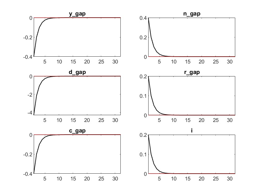
stoch_simul(order=1, irf=32) y_gap w_gap n_gap d_gap r_gap c_gap i;
This is a replication of the Paper “The New Keynesian Transmission Mechanism: A Heterogenous Agent Perspective” by Broer et al. In this case the classical textbook NK model (RANK) is tested under flexbile wages and rigid prices. In the paper the IRF for the variables of interest (y_gap, w_gap, n_gap: as change of hours worked, d_gap, r_gap, c_gap, i) that Inflation, Consumption gap, output gap, employement gap, real wage gap react negativ, real interest rate gap and profit gap react positiv. But in my calculations output, profits consumption react negative and inflation, real interest rate gap and employement react positive. where could the problem arise? given those equations:
Monetary policy (Taylor rule)
Representative‐Agent (RANK)
Consumption Euler
NK Phillips (goods
Wage‐inflation Phillips:
Intratemporal:
Market clearing: