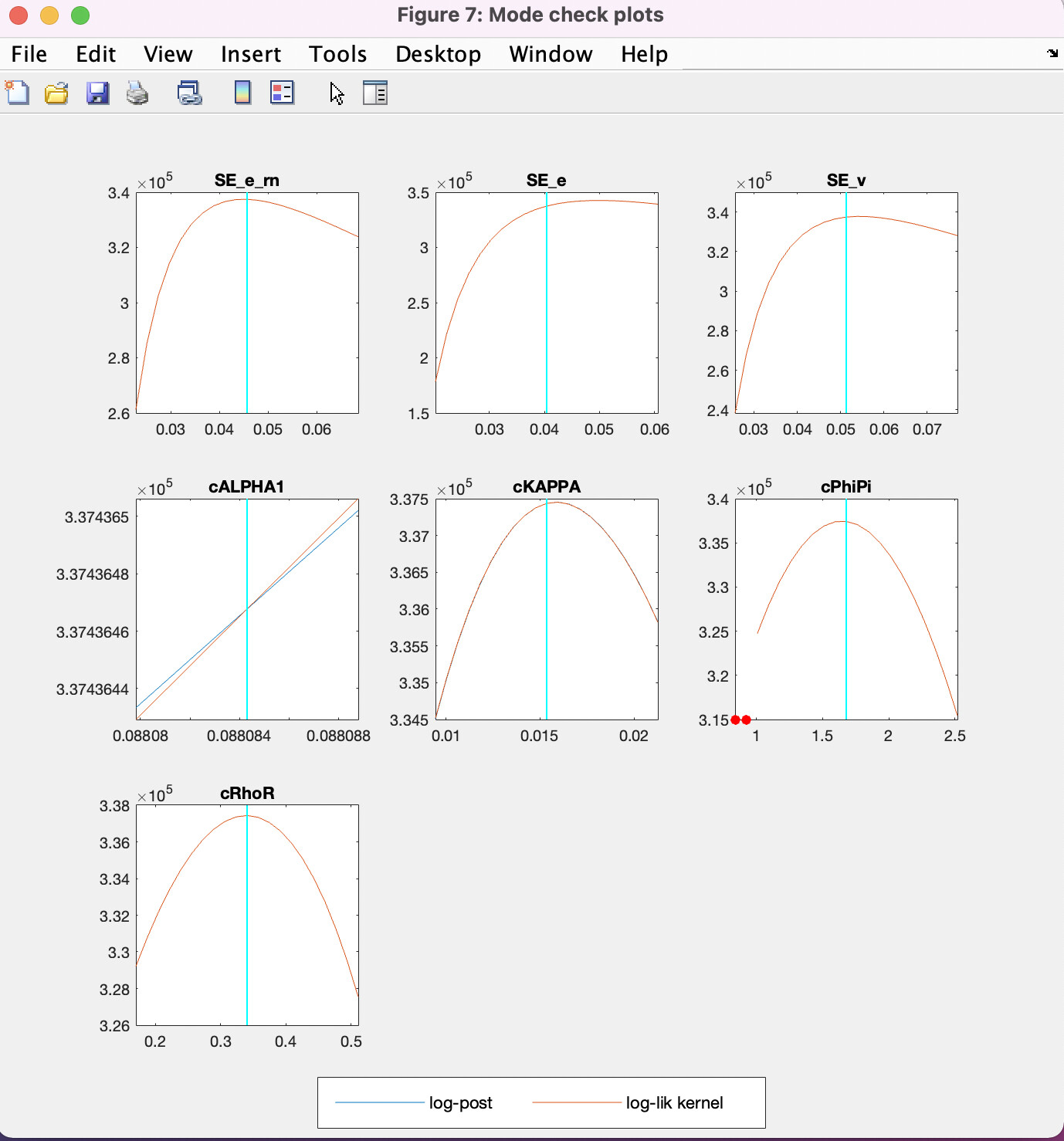
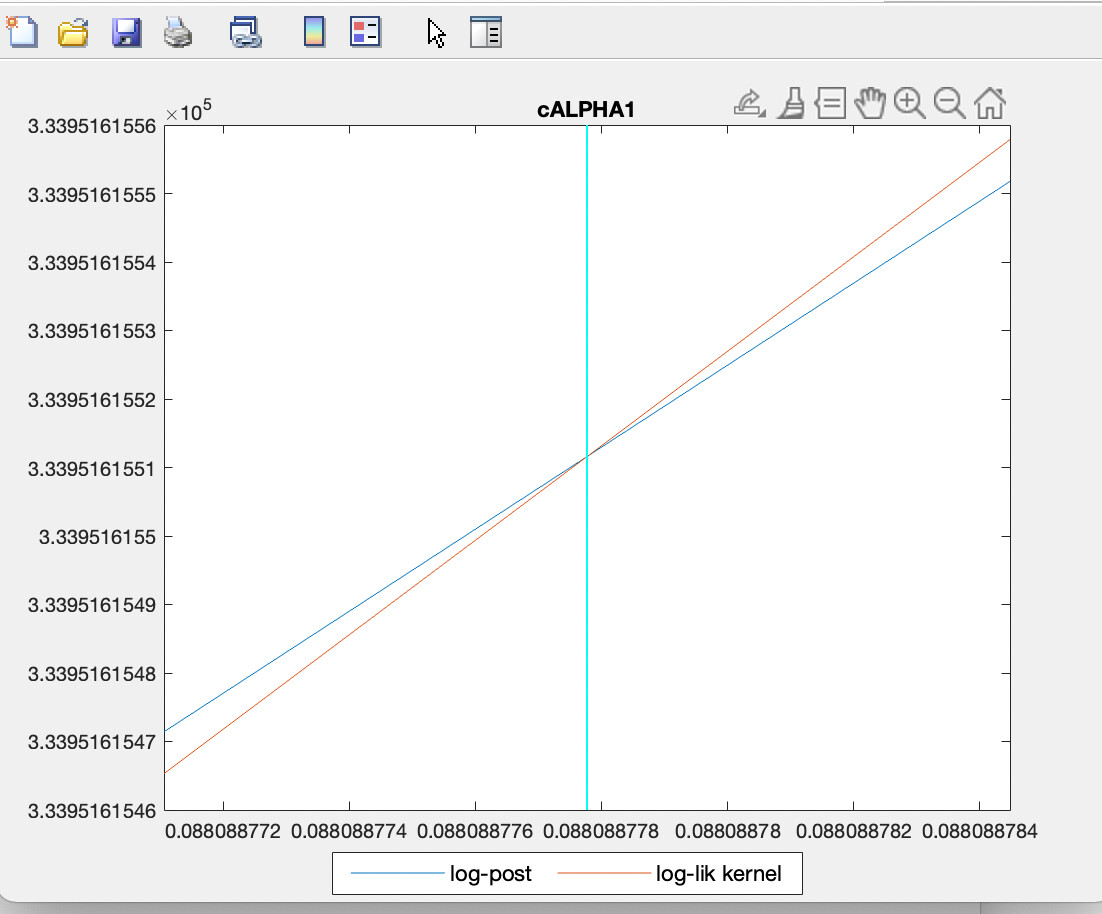
What is happening when x_axis and y_axis are both very tight (for cALPHA1)?
As far as I know, this is due to some necessary conditions like B-K in some cases, but it seems not to be the case in this case. (too tight, and for example, cALPHA1 = 0.1 can satisfy B-K.)
I also thought this is because other parameters are bounded by some conditions but this was not the case, since even though I estimate only one parameter, almost the same graph was obtained.
Usually that happens if the parameter runs extremely close to its bounds.
Is this "extremely close to its bound " implying that B-K or other necessary conditions seem to be violated around 0.088088? In my expectation, this parameter can be at least any value between 0 ~ 0.11… Or, does it imply completely other things?
Did you set prior_trunc=0 ?
I did not change from its default(1e-32). By changing it to 0, I managed to obtain fine result! However, why does the change solve the issue?
I’ve read official document and some questions here, but I didn’t figure out how they are related. ( My understanding is that by lowering prior_trunc to 0, we can catch a parmeter_vector which happens very low probability, but mode should not be such a point.(since it should happen most often, generally.)
Being close to BK condition violations would usually show up in the mode_check-plots as red dots.
What you experience is more likely being close to the bound introduced by prior_trunc. That option cuts off the very thin tails of the prior distributions. But that means the bounds used internally can differ from the explicit bounds you have in mind. That may be the case for you.
You are right that usually the mode should not be in the regions where you assign a very low prior probability. But in rare cases that may happen. If we know what the data tell us, we would not need to estimate a model.
Thank you very much! Your comments are very helpful!
With respect to 2., 3, I guess I understood what was happening in my default prior_trunc.
Now, my question is whether the narrow x-axis implies the range dynare managed to compute is just it(in the case of the picture2, a very narrow range around 0.088), or not? (just because Dynare is focusing on the narrow range.)
I’m checking oo_.posterior, but I couldn’t find the raw log-posterior distribution data.
You did not yet compute oo_.posterior, only the mode. Thus, you cannot look at it yet.
The narrow range comes from Dynare plotting a neighborhood around the detected mode. If you run into a bound on one side, e.g. due to prior_trunc that typically results in the narrow x-range. That is why I have been pointing this out from the start.
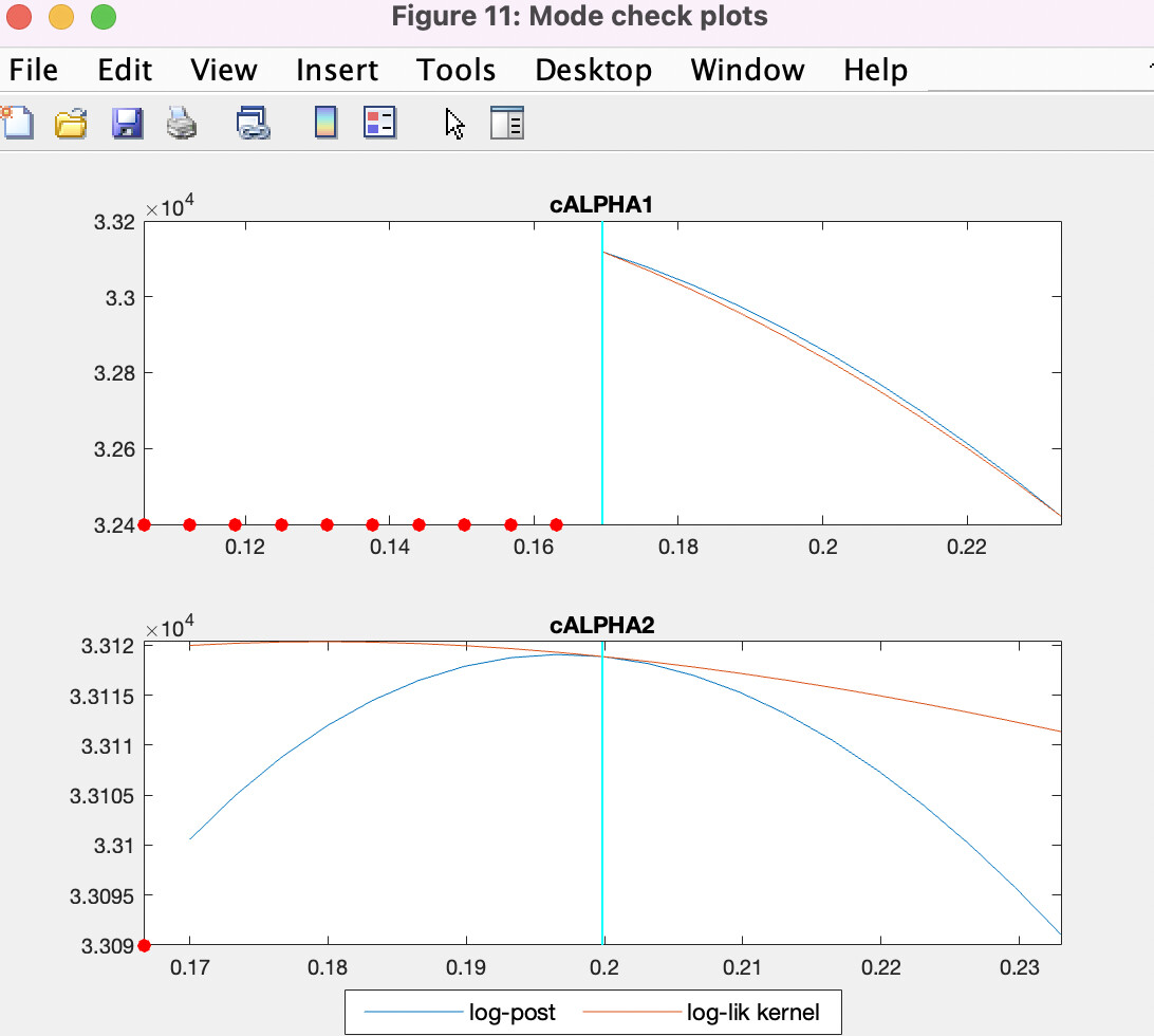
Now, I’m estimating with simulated 1000 periods fake data for a model.
I set cALPHA2 as 0.1 when it is generated, and I set prior distribution for estimation as uniform distribution from -0.2 to 0.9.
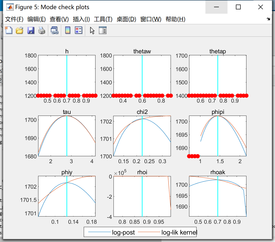
However, I had a Mode check plots below.
Is this just because data is not enough or the parameter cannot be identified and estimation is failing?
Or, is there possibility that I can get fine estimation result by trying other options? (eg. changing prior_trunk, mode_compute etc)
In my understanding, even if I change the way to calculate mode, the result cannot be better, because log-like kernel is already obvious wrong. (I tried something and this thought seems right, but I cannot try all the options, so I’m not confident.)
Is this thought right?
Dear, professor.I performed normal Bayesian estimation, and the distribution of estimated parameters also referred to mainstream literature, but I still encountered red dot errors when estimating parameters. I don’t know what’s wrong with the model. please help me~ bayes.mod (12.0 KB)
How can I solve this problem. I did not find error about the model. Do you mean that my steady-state solution is wrong, but if I don’t calibrate the parameters with the red dots, the model will work
if there are red dots on the mode_check plots, does this mean the parameter estimation is wrong? if not, what kind of information we can get from the red dots? How shoudl we deal with the red dots?
Thank you Prof. Pfeifer for answering my question. You mentioned “When adding options_.debug=1 you will get information where the red dots in the mode_check-plots come from.” How to add this? Do you mean Just add options_.debug=1 inside the estimation() command? like we add mode_check inside the estimation() command