Hi everyone,
I am working on a nonlinear NK-DSGE model with two energy sectors (brown and green), a CES energy aggregator, Rotemberg price adjustment in both energy sectors and the final-goods sector, and government investment in brown and green energy capital.
I have attached:
- Paper2_V9.mod
- paper2_V9_steadystate.m
- All my model equations
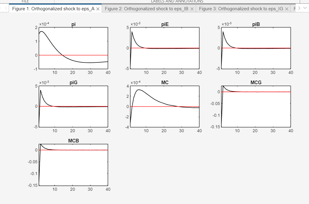
- An example of the IRFs I am currently getting
The steady state file runs, but the model is not properly closed. My issue is that I appear to be missing one independent equation, but many candidate equations I try become collinear with existing equations.
The problem seems to be in the energy-price / energy-aggregator block.
My current energy aggregator block is:
\begin{align}
E_t &= \left[\phi_E(\chi_t^G)^{\frac{\sigma-1}{\sigma}} + (1-\phi_E)(\chi_t^B)^{\frac{\sigma-1}{\sigma}}\right]^{\frac{\sigma}{\sigma-1}}\\
\chi_t^G &= \phi_E^\sigma \left(\frac{q_t}{F(q_t)}\right)^{-\sigma} E_t\\
F(q_t) &= \left[\phi_E^\sigma q_t^{\,1-\sigma} + (1-\phi_E)^\sigma \right]^{\frac{1}{1-\sigma}}\\
q_t &= \frac{\pi_t^G}{\pi_t^B} q_{t-1}\\
\pi_t^E &= \pi_t^B \frac{F(q_t)}{F(q_{t-1})}\\
P_t^E &= \frac{\pi_t^E}{\pi_t}P_{t-1}^E
\end{align}
Then in the intermediate-goods block I use:
P_t^E = MC_t (1-\alpha_L-\alpha_K)\frac{Y_t} {E_t}
So P_t^E is being treated as the real relative price of the composite energy input.
My suspicion is that the problematic equation is:
P_t^E = (\pi_t^E/\pi_t) P_{t-1}^E
I believe this is the wrong closure, but I have not been able to identify the correct replacement.
What I have already tried / ruled out:
- Adding the brown-energy demand equation from the CES aggregator
- Adding explicit marginal-cost level equations for MC_t^B and MC_t^G
- Adding the aggregate resource constraint
In each of those cases, Dynare solves the steady state but reports collinearity.
I need help identifying is:
- In this current setup, is there one genuinely missing independent equation?
- If so, which equation is the correct one to replace
P_t^E = (\pi_t^E/\pi_t) P_{t-1}^E ?
- Or alternatively, is the issue that one of my existing equations is redundant/mis-specified, so that the model is rank-deficient rather than simply “missing” an equation?
From the image you can see that the equation P_t^E = (\pi_t^E/\pi_t) P_{t-1}^E cause a 1 period weird jump in my IRFs. This is why I think it is the problem equation in the model.
Any guidance on the correct closure of the energy price block would be greatly appreciated. Or any guidance on where I am implementing something incorrectly.
Paper2_V9.mod (10.3 KB)
paper2_V9_steadystate.m (11.2 KB)
The complete model setup
The equilibrium process in a symmetric equilibrium is described by the following endogenous variables:
\{
C_t, I_t, r_t, K_t, \pi_t, W_t, L_t, \Psi_t, T_t, \Omega_t^K, \lambda_t, \lambda_t^K, \chi_t^B, A_t, M_t, K_t^B, Z_t, U_t, \varphi_t, \Xi_t,
C_{A,t}, p_t^B, \Psi_t^{\chi,B}, r_t^B, \pi_t^B, \tau_{Z,t}, MC_t^B, \Omega_t^B, \chi_t^G, p_t^G, K_t^G, \Psi_t^{\chi,G}, r_t^G, \pi_t^G, MC_t^G,
\Omega_t^G, E_t, q_t, \pi_t^E, Y_t, P_t^E, MC_t, \Omega_t, G_t, I_t^E, I_t^G, I_t^B, I_t^{B,K}, I_t^{B,\Xi}, \Omega_t^{B,K}, \Omega_t^{G,K}
\}
Households
\begin{aligned}
C_{t} + I_{t} &= \frac{r_{t-1}K_{t-1}}{\pi_{t}} + W_tL_{t} + \Psi_t - T_t \\
K_{t} &= (1 - \delta)K_{t-1} + (1- \Omega_{t}^K)I_{t} \\
\lambda_{t} &= (C_{t} - hC_{t-1})^{-1} - \beta h \mathbb{E}_t(C_{t+1} - hC_{t})^{-1} \\
\lambda^{K}_t &= \beta\mathbb{E}_t[\lambda_{t+1}\frac{r_{t}}{\pi_{t+1}} + \lambda_{t+1}^{K}(1 - \delta)]\\
\lambda_{t} &= \lambda_{t}^{K}[1 - \Omega_{t}^K - \Omega_{t}^{K'}I_{t}] - \beta\mathbb{E}_t[\lambda_{t+1}^{K}\Omega_{t+1}^{K'}I_{t+1}]\\
\lambda_{t}W_t &= \gamma(1 - L_{t})^{-1}\\
\Omega_t^K &\equiv (\Omega^K/2)[(I_{t}/I_{t-1}) - 1]^2\\
\Omega^{K'}_t &\equiv (\Omega^K/I_{t-1})[(I_{t}/I_{t-1}) - 1]\\
\Omega^{K'}_{t+1} &\equiv \Omega^K [(I_{t+1}/I_{t}) - 1](\frac{-I_{t+1}}{I_{t}^2})
\end{aligned}
Energy Producers
Brown energy producer
\begin{aligned}
\chi_{t}^B &= A_t(1 - \Gamma(M_t))(K^B_{t-1})^{\alpha_B}\\
\Gamma(M_t) &= \gamma_0 + \gamma_1 M_t + \gamma_2 M_t^2 \\
M_{t} &= (1-\delta_M)M_{t-1} +Z_{t} \\
Z_{t} &= (1 - U_{t})\varphi_t \chi_{t}^B\\
\varphi_t &= \varphi \exp(-\upsilon \Xi_{t-1})\\
C_{A,t}(U_{t},\chi_{t}^B) &= \phi_1(U_{t})^{\phi_{2}}\chi_{t}^B\\
p_t^B &= \frac{P_t^E}{\left[\phi_E^\sigma q_t^{1-\sigma} + (1-\phi_E)^\sigma\right]^{\frac{1}{1-\sigma}}}\\
\Psi_t^{\chi,B} &= p_t^B\chi_t^B - p_t^B\frac{r_{t-1}^BK_{t-1}^B}{\pi_t^B} - C_{A,t} - \tau_{Z,t}Z_t - p_t^B\Omega_t^B\chi_t^B \\
\frac{r^{B}_{t}}{\pi^B_{t+1}} &= MC^B_{t+1}\alpha_B\frac{\chi_{t+1}^B}{K^B_{t}} \\
\varphi_t \tau_{Z,t} &= \phi_{1}\phi_{2}(U_{t})^{\phi_{2} - 1} \\
\Omega^B_t &= (\Omega_B/2)[\frac{\pi_t^B}{\pi^B} - 1]^{2} \\
\Omega^B(\frac{\pi_t^B}{\pi^B} - 1)\frac{\pi_t^B}{\pi^B} &= \beta\mathbb{E}_t\left[\frac{\lambda_{t+1}}{\lambda_t}\Omega^B(\frac{\pi_{t+1}^B}{\pi^B} - 1)\frac{\pi_{t+1}^B}{\pi^B}\frac{\chi_{t+1}^B}{\chi_t^B}\right] + \epsilon_B MC_t^B + (1 - \epsilon_B)
\end{aligned}
Green energy producer
\begin{aligned}
\chi_{t}^G &= A_t(1 - \Gamma(M_t))(K^G_{t-1})^{\alpha_G}\\
p_t^G &= q_t p_t^B\\
\Psi_t^{\chi,G} &= p_t^G \chi_t^G - p_t^G \frac{r_{t-1}^G K_{t-1}^G}{\pi_t^G} - p_t^G \Omega_t^G \chi_t^G\\
\frac{r^{G}_{t}}{\pi^G_{t+1}} &= MC^G_{t+1}\alpha_G\frac{\chi_{t+1}^G}{K^G_{t}} \\
\Omega^G_t &= (\Omega_G/2)[\frac{\pi_t^G}{\pi^G} - 1]^{2} \\
\Omega^G(\frac{\pi_t^G}{\pi^G} - 1)\frac{\pi_t^G}{\pi^G} &= \beta\mathbb{E}_t\left[\frac{\lambda_{t+1}}{\lambda_t}\Omega^G(\frac{\pi_{t+1}^G}{\pi^G} - 1)\frac{\pi_{t+1}^G}{\pi^G}\frac{\chi_{t+1}^G}{\chi_t^G}\right] + \epsilon_G MC_t^G + (1 - \epsilon_G)
\end{aligned}
Energy aggregator
\begin{aligned}
E_t &= \left[\phi_E(\chi_t^G)^{\frac{\sigma-1}{\sigma}} + (1-\phi_E)(\chi_t^B)^{\frac{\sigma-1}{\sigma}}\right]^{\frac{\sigma}{\sigma-1}}\\
\chi_t^G &= \phi_E^\sigma \left(\frac{q_t}{F(q_t)}\right)^{-\sigma} E_t\\
F(q_t) &= \left[\phi_E^\sigma q_t^{\,1-\sigma} + (1-\phi_E)^\sigma \right]^{\frac{1}{1-\sigma}}\\
q_t &= \frac{\pi_t^G}{\pi_t^B} q_{t-1}\\
\pi_t^E &= \pi_t^B \frac{F(q_t)}{F(q_{t-1})}\\
P_t^E &= \frac{\pi_t^E}{\pi_t}P_{t-1}^E
\end{aligned}
Intermediate good firms
\begin{aligned}
Y_{t} &= (1 - \Gamma(M_t))A_t(L_{t})^{\alpha_L}(K_{t-1})^{\alpha_K}(E_{t})^{1 - \alpha_L - \alpha_K}\\
\Psi_t &= Y_t - W_t L_t - \frac{r_{t-1} K_{t-1}}{\pi_t} - P_t^E E_t - \Omega_t Y_t \\
\frac{r_{t}}{\pi_{t+1}} &= MC_{t+1}\alpha_K\frac{Y_{t+1}}{K_{t}} \\
W_t &= MC_t\alpha_{L}\frac{Y_{t}}{L_{t}} \\
P_{t}^{E} &= MC_t (1 - \alpha_L - \alpha_K)\frac{Y_{t}}{E_{t}} \\
\Omega_t &= (\Omega/2)[\frac{\pi_t}{\pi} - 1]^{2} \\
\Omega(\frac{\pi_t}{\pi} - 1)\frac{\pi_t}{\pi} &= \beta \mathbb{E}_t\left[\frac{\lambda_{t+1}}{\lambda_t}\Omega(\frac{\pi_{t+1}}{\pi} - 1)\frac{\pi_{t+1}}{\pi}\frac{Y_{t+1}}{Y_t}\right] + \omega MC_t + (1 - \omega)
\end{aligned}
Government and environmental regime
\begin{aligned}
G_t + I_t^E &= T_t + p_t^B \frac{r_{t-1}^B K_{t-1}^B}{\pi_t^B} + p_t^G \frac{r_{t-1}^G K_{t-1}^G}{\pi_t^G} + \Psi_t^{\chi,B} + \Psi_t^{\chi,G}\\
G_{t} &= gY_{t}\\
I_{t}^{E} &= [\kappa(I_{t}^{G})^{\frac{\varsigma-1}{\varsigma}} + (1-\kappa)(I_{t}^{B})^{\frac{\varsigma-1}{\varsigma}}]^{\frac{\varsigma}{\varsigma-1}}\\
I_t^{B,K} &= (1-\xi) I_t^B \\
I_t^{B,\Xi} &= \xi I_t^B + \frac{\tau_{Z,t}Z_t}{2} \\
K^B_{t} &= (1 - \delta_B)K^B_{t-1} + (1- \Omega^{B,K}_{t})I^{B,K}_{t} \\
\Xi_t &= (1-\delta_\Xi)\Xi_{t-1} + I_t^{B,\Xi} \\
\Omega^{B,K}_t &\equiv (\Omega^{B}/2)[(I^{B,K}_{t}/I^{B,K}_{t-1}) - 1]^2\\
K_t^G &= (1-\delta_G)K_{t-1}^G + (1-\Omega_{t}^{G,K})I_{t}^G + \frac{\tau_{Z,t}Z_t}{2}\\
\Omega_t^{G,K} &\equiv \frac{\Omega^{G,K}}{2}\left[\left(\frac{I_t^G}{I_{t-1}^G}\right)-1\right]^2\\
\frac{1 + r_{t}}{1 + r} &= \left(\frac{\pi_t}{\pi}\right)^{\theta_{\pi}} \left(\frac{\pi_t^E}{\pi^E}\right)^{\theta_E} \left(\frac{Y_t}{Y}\right)^{\theta_Y}
\end{aligned}
Model shocks
\begin{aligned}
\log (A_t) &= (1-\rho_A)\log (A) + \rho_A\log (A_{t-1}) + \epsilon_{A,t}\\
\log (I_{t}^B) &= (1-\rho_{I^B})\log (I^B) + \rho_{I^B}\log (I_{t-1}^B) + \epsilon_{I^B,t}\\
\log (I_{t}^G) &= (1-\rho_{I^G})\log (I^G) + \rho_{I^G}\log (I_{t-1}^G) + \epsilon_{I^G,t}\\
\log (\tau_{Z,t}) &= (1-\rho_{\tau_{Z}})\log (\tau_Z) + \rho_{\tau_{Z}}\log (\tau_{Z,t-1}) + \epsilon_{\tau,t}
\end{aligned}