Long lasting deterministic transitory shocks vs true permanent: what is happening?

[frafer]

Hello Dynare programmers,

I am currently working with a highly non-linear energy model, and I am trying to obtain the transition dynamics to a perfect foresight deterministic shock. Specifically, I want to increase emission taxes linearly for 32 years and keep the tax value constant after period 32.

I have encountered some difficulties with the nonlinear solver while trying to obtain the solution for the required size of the shock, and I have only been able to obtain a solution for a shock about one-third of the required size.

To verify my results, I compared the nonlinear solution with the one obtained using the ‘linear_approximation’ option, which first linearizes the model. They are almost identical. I then used the ‘linear_approximation’ option to obtain the solution for the required shock size, which I believe should be very similar to the nonlinear solution.

My first question is: Am I correct in assuming that the linearized solution should be very similar to the nonlinear solution for the type of simulation I am doing?

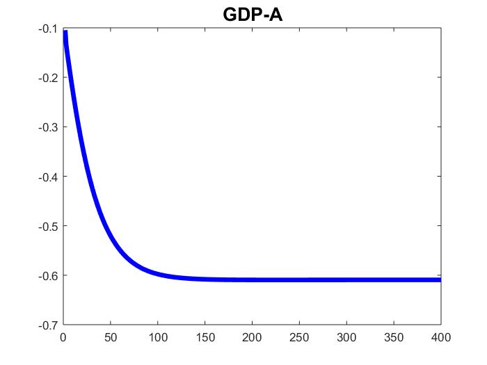
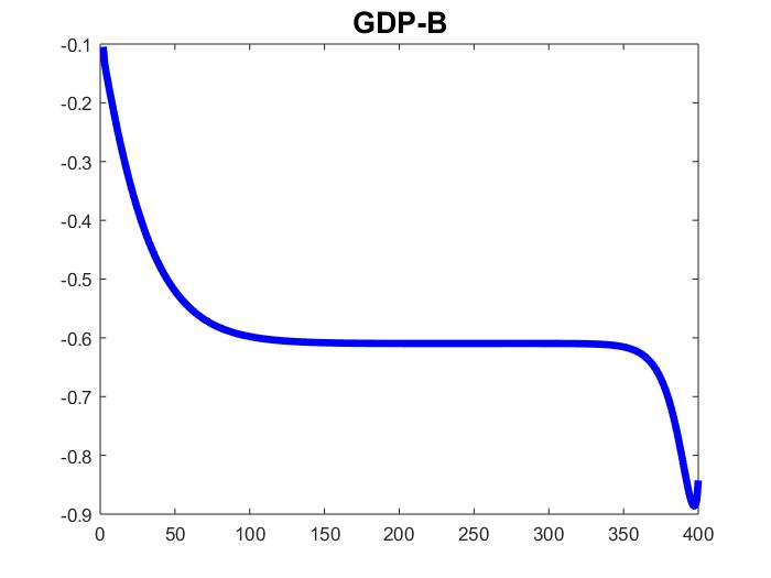
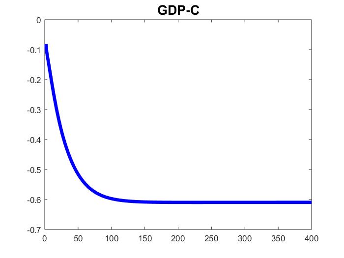
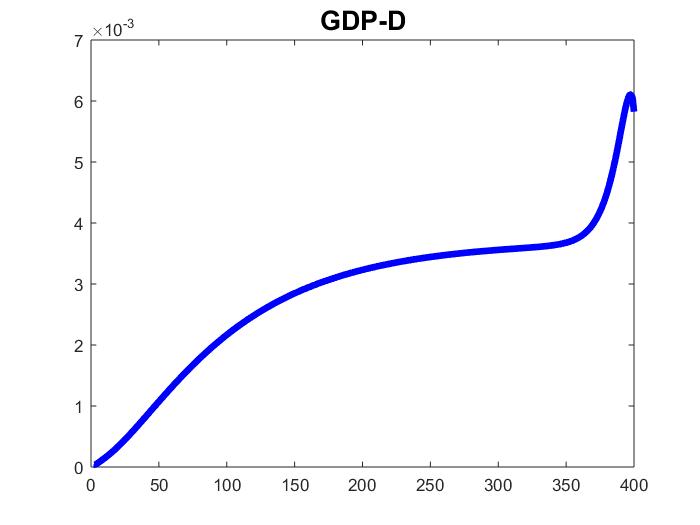
My second question is a bit more tricky. I noticed that the dynamic solution I obtained for the first 10 periods is significantly different when I implement the perturbation using a transitory shock lasting 400 periods (in which the exogenous variable increases linearly during the first 32 periods and remains constant afterward) compared to when I use the ‘endval’ for a permanent shock combined with the same transitory shock.

Given the long duration of the transitory shock, I expected the impact of the perfect foresight exogenous variable after period 400 to have a negligible effect on the dynamic solution for the first 10 periods. However, the difference between the two methods is significant. Additionally, the solution for the long-lasting transitory shock is mathematically inconsistent. Specifically, when I feed one equation of the model with the dynamic solution of the implied endogenous variables, the values I obtain for the endogenous variables in the left-hand side do not coincide with those displayed by Dynare.

Therefore, my second question is: Why am I obtaining very different solutions between the two methods, and why is the solution for the long-lasting transitory shock mathematically inconsistent?

More formally, shocking the model as in (A) or (B) below displays very different solutions:

(A) minc = 61.43*3.67/1000; % Baseline

endval;

tauini = minc;

end;

steady;

shocks;
var tauini;
periods 1:32 33:400;
values (linspace(0,minc,32)) (linspace(minc,minc,400-32));
end;

(B) minc = 61.43*3.67/1000; % Baseline

shocks;
var tauini;
periods 1:32 33:400;
values (linspace(0,minc,32)) (linspace(minc,minc,400-32));
end;

I provide the files you need to run the model.

Thank you in advance for your very useful comments.

param_g_b.mat (375 Bytes)
ss_g_b.mat (536 Bytes)
Model_g_b_emission_tax_help.mod (11.9 KB)

[jpfeifer]

1. For small shocks, you would expect both to be quite similar. But the quality of the approximation will deteriorate, the bigger the shocks and the bigger the persistence, because you move further away from the approximation point.

2. For the second point, it is hard to understand what is going on. I would need to see the two different implementation files. My hunch is that it has to do with the call to steady after endval, which will determine the values for the terminal condition of the forward-looking variables. Put differently, I think the terminal conditions used in the two simulations differ.

[frafer]

Thank you so much , Prof. Pfeifer, for your response.

1. That
   Model_g_b_lasting.mod (11.9 KB)
   Model_g_b_permanent.mod (11.9 KB)
   was also my guess.

As for 2., I attach two files, the only difference is that in one the shock is of long duration (400 periods) while in the other it is permanent. Notice how much the results differ.

[frafer]

Note also that if you reduce the size of the shock to very small, long-duration exercise still gives weird results.

[jpfeifer]

The difference is indeed caused by not properly setting the terminal condition. You set an identical exogenous process, but not the same terminal condition.

[frafer]

Thank you for your response. As I understand the terminal condition is properly set. Take the case of a shock of a size 0.000001. If this shock is truly permanent the terminal condition is 0.000001 whilst if it is just long lasting the terminal conditon is just 0. Is that enough to provoke such a big changes in the dymanics of the the first periods?

[jpfeifer]

If I set minc = 0.0001; % Baseline the two approaches return virtually identical results.

[frafer]

Upss! I don’t get that. Actually, with minc = 0.0001 the solution for the long.lasting:

erfect foresight solution found.

emissions change (%) by 2050

ans =

-2.1190e+05

tax on CO2 tonnes by 2050 (euros)

ans =

0.2725

Abatment (share in %)

ans =

1.0e+04 *

0.0000
0.0000
0.7063
1.4127
2.1190
2.8253
3.5317
4.2380
4.9443
5.6507

And the solution for the true permanent:

Perfect foresight solution found.

emissions change (%) by 2050

ans =

-0.2762

tax on CO2 tonnes by 2050 (euros)

ans =

0.0272

Abatment (share in %)

ans =

0.0000
0.1159
0.1206
0.1252
0.1299
0.1346
0.1393
0.1439
0.1486
0.1533

[frafer]

Model_g_b_permanent.mod (11.9 KB)
Model_g_b_lasting.mod (11.9 KB)

[jpfeifer]

My hunch is the problem is not having called steady for your terminal condition. That implies the initial steady state is the approximation point used. That should matter much in your context. Use

rplot tauini mu_b;

to see the very different trajectories in the two cases (including the strange terminal condition you are getting in the lasting case). Here, the system never settles to a terminal steady state.

[frafer]

Thank you, Prof Pfeizer. Actually this problem does not occur when I use the nonlinear solver, so it seems it has to do with which steady state the solver is taking for the approximation point (the initial or the final). As I understand the terminal condition problem would apply also for a nonlinear solver, but I said, in this cas it is not a problem anymore. For the exercises I am doing it makes more sense approximate around the initial steady state which take us back to the initial question, why a linear approximation then provokes such as weird results.

The problem repeats for other different experiments: as I use a linear approximation, a long lasting constant shock produces very different short run results than a true permanent shock. An this does not happen with the nonlinear solution.

[jpfeifer]

But do you really implement a steady state as the terminal condition in both cases you are comparing?

[frafer]

Let’s consider four cases:

A) Starting from x0, nonlinear solution with a permanent deterministic ‘shock’ of size k, and with a terminal condition x0 +f.
B) Starting from x0, nonlinear solution with a long lasting ‘shock’ of size k, and with a terminal condition x0.
C) Starting from x0, linear solution with a permanent ‘shock’ (k) with a terminal condition x0+f.
D) Starting from x0, linear solution with a long lasting ‘shock’ (k) with a terminal condition x0.

What I find is that the dynamic solution for (A) and (B) is identical except for the periods close to the the terminal condition. Actually, for the case (B), if I prolong the shock quite enough on time (from t0 to m) , then the dynamic solution corresponding to period t0+s (where s is very large, and m-s=n is also large enough) coincides with the new steady state solution in (A).

I also find that dynamic solution in (C) is very similar (although) non identical to (A), and (B), as we would expect from a linear approximation.

However, the dynamic solution in (D) is completely different from that in the three previos cases, and I would like to know what explains this difference.

[jpfeifer]

Does case D) show a gradual return to the initial steady state x0?

[frafer]

Please, see these plots for the behaviour of GDP in an exercise of the four different cases. For cases B and D the shock lasts 400 periods. A and B are non linear solutions, and C and linear solutions. A and C are pure permanent shocks with the same terminal condition, and B ad D long lasting shocks with a terminal condition different from A and C. Notice that I obtain the same dynamic solution during (say) the first 100 periods in A and B. I can also ‘recover’ the new steady state from B if I look at (say) period 200 (wich coincides with the new steady state in A). Notice also that case C is virtually the same as A. However, case D is completely different.

[frafer]

[frafer]

[frafer]

[frafer]

[jpfeifer]

You need to conduct proper simulations, i.e. leave enough time for the system to settle to its terminal steady state. That is not the case for B and D.