Intraperiod loan in the NK model

[Victory10]

Hello!

I have constructed a simple NK model that includes a household sector, an intermediate goods sector, an aggregated goods sector, the government, and the central bank. Households interact with the production sector by supplying labor to intermediate firms. Their interaction with the government occurs through the purchase of bonds, from which they earn interest income. The central bank sets the interest rate.

Intermediate goods producers interact with households by paying wages and distributing profits. The aggregation sector combines various intermediate goods into a single final good, which is then allocated for household and government consumption as well as investment. Additionally, firms own capital.

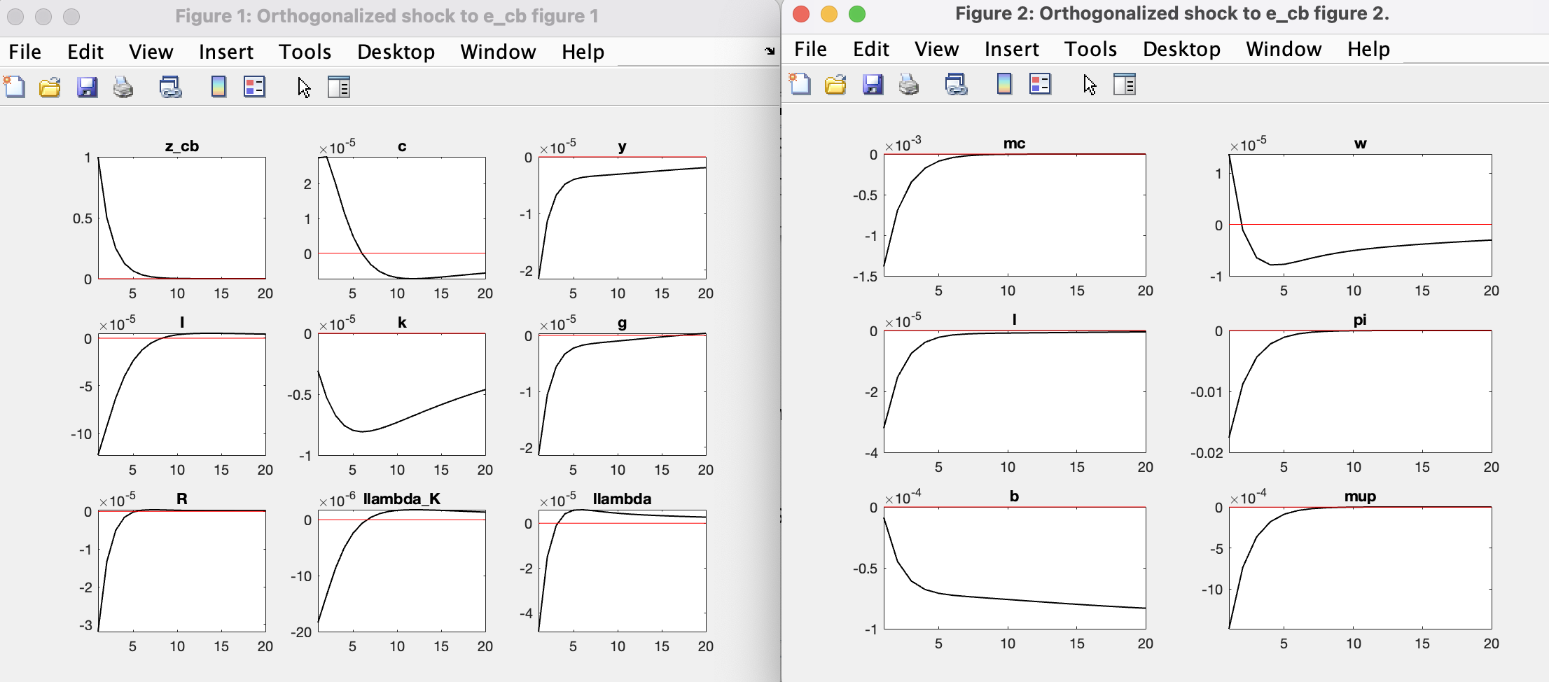
I am trying to introduce a borrowing constraint for the production sector (intraperiod loan) into the model, following the approach of Sims (2017) (https://sites.nd.edu/esims/files/2023/05/financial_constraint_2017.pdf). However, when I incorporate this constraint and analyze a positive monetary shock, I observe an unexpected outcome: instead of rising sharply, the interest rate drops significantly in response to the shock, even though the shock is applied directly to the central bank’s policy rate. Without the constraint, the interest rate responds to a positive monetary shock by increasing.

The monetary policy shock is specified as:
z_cb = rhocb * z_cb(-1) + e_cb;
And the central bank’s interest rate rule is:
R/STEADY_STATE(R) = (R(-1)/STEADY_STATE(R))^rhocb * (((pi / STEADY_STATE(pi))^(gamma_cb))^(1 - rhocb)) + z_cb;

Could you help me understand why this is happening?

[jpfeifer]

Positive monetary policy shock with nominal interest rate falling? - #4 by jpfeifer may be relevant.

[Victory10]

Thank you very much!

[Victory10]

Dear Professor @jpfeifer,

I have incorporated an intertemporal credit constraint into my model of the following form:
D_{t+1}(j) \leq \xi_t \lambda_t^K K_{t-1}(j)

where investment is fully financed by new one-period debt, i.e., (I_t(j) = D_{t+1}(j)). This constraint implies that firms finance their investment entirely through the issuance of short-term debt backed by the value of their capital.

I am currently analyzing forward guidance policy under persistently high interest rates. My hypothesis is that, as the central bank continuously raises the interest rate, firms’ demand for credit increases, since agents anticipate even higher rates in the future.

Could you please advise on how to modify the credit constraint to capture this mechanism? Specifically, how can I incorporate agents’ expectations so that higher current interest rates lead to greater borrowing today, due to expectations of even higher rates tomorrow?

Thank you very much in advance!

[Victory10]

Dear Professor @jpfeifer,

I’m trying to incorporate something like the difference between the expected interest rate and the current interest rate into this borrowing constraint. However, I’m not quite sure how to do this properly. I would really appreciate your guidance if you have any ideas on how this could be implemented.

Thank you very much in advance!

[jpfeifer]

I guess the typical way is to have a standard constraint of the form you mentioned. The intertemporal substitution usually comes from the forward looking Euler equations.

[Victory10]

Dear Professor @jpfeifer,

Thank you very much for your response.

I’m a bit confused and would appreciate some clarification. Am I correct in understanding that I should include the difference between the expected and the current interest rate directly into the standard borrowing constraint for firms? Something like:
I_t(j) \leq \xi_t \lambda_t^K K_{t-1}(j) + E_t R_t - R_{t-1}

Also, should I then derive the corresponding Euler equation from the firm’s optimization problem? I’m asking because the usual Euler equation is derived from household consumption decisions, whereas in this case, we are talking about borrowing constraints, which – at least in my interpretation – relate to investment behavior.

Does that mean I should derive the Euler equation using the first-order conditions with respect to capital and investment? For reference, here are the first-order conditions I’m using in my model:

\frac{∂L(j)}{∂K_t(j)} = -\lambda_t^K + β E_t \left( \frac{\lambda_{t+1}}{\lambda_t} \left[ \lambda_{t+1}^K \left( (1 - δ) + ψ^I \frac{I_{t+1}(j)}{K_t(j)} \left( \frac{I_{t+1}(j)}{K_t(j)} - δ \right) - \frac{ψ^I}{2} \left( \frac{I_{t+1}(j)}{K_t(j)} - δ \right)^2 + μ_{t+1} ξ_{t+1} \right) \right] + αP_{t+1}(j) A_{t+1}(L_{t+1}(j))^{1 - α} K_t(j)^{α - 1} \right) = 0

\frac{∂L(j)}{∂I_t(j)} = \lambda_t^K \left( 1 - ψ^I \left( \frac{I_t(j)}{K_{t-1}(j)} - δ \right) \right) - μ_t - β E_t \left( \frac{\lambda_{t+1}}{\lambda_t} R_t \right) = 0

In my model, I’ve been analyzing forward guidance under the usual constraint
I_t(j) \leq \xi_t \lambda_t^K K_{t-1}(j)
using a long horizon:

var e_cb; periods 8:40; values 0.0025;  

However, I haven’t observed the kind of results I expected – specifically, the idea that higher current interest rates would lead firms to borrow more now, anticipating even higher rates in the future.

I would be very grateful for any thoughts or guidance you might have on how to approach this.

[jpfeifer]

1. What would be the justification for including that term in the constraint?
2. The investment/savings decision is the counterpart of the consumption decision. Usually, it governs both.
3. With future shocks there is usually a tradeoff between income/wealth effects and substitution effects. If the former dominate, you may not see the desired intertemporal substitution you expect.

[Victory10]

Professor @jpfeifer, sorry to bother you again. If I understand correctly, I should focus on reducing the dominance of the income/wealth effect in my model? So I need to work on the calibration and/or the Euler equation? But I’m still a bit confused about the Euler equation in this case, since in my model it’s the firms who make investment decisions, not households.

[jpfeifer]

The firm’s investment decision is nevertheless an Euler equation as it links today’s and tomorrow’s objective functions.
My point is more general: try to understand the intertemporal dynamics and whether they can deliver the expected result. For example, there is an older literature on the effect of anticipated tax shocks and the features required there to get data consistent behavior were rather complex. I am referring the Mertens/Ravn work, where depreciation allowances were absolutely key (which was non-obvious from the start). Coming up with a good model is hard.

[Victory10]

Professor, thank you very much for your answers!