Interest rate rule about GK_2011

[max3]

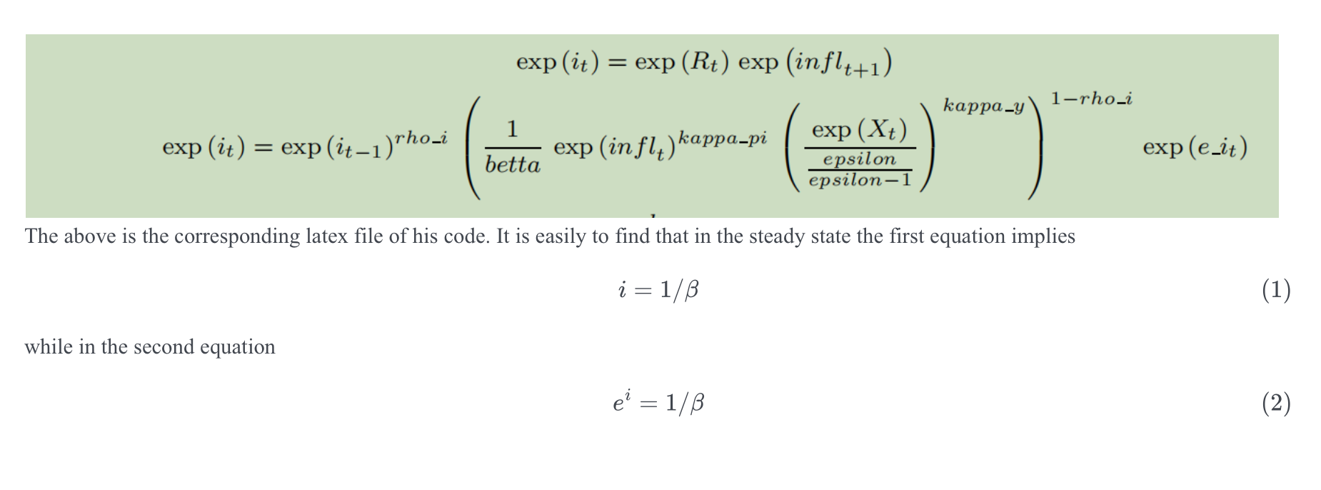
Hello everyone, I’ve been recently replicating the GK-2011 paper and encountered some confusion when dealing with nominal interest rates and interest rate rules.In his paper, the nominal interest rate is net,

i_t=(1-\rho)\left[\frac{1-\beta}{\beta}+\kappa_\pi \pi_t+\kappa_y\left(\log Y_t-\log Y_t^*\right)\right]+\rho i_{t-1}+\varepsilon_t\\ 1+i_t=R_{t+1} \frac{E_t P_{t+1}}{P_t}

If we define $i_t$​ is gross nominal interest rate , then

i_t=(1-\rho)\left[\frac{1}{\beta}+\kappa_\pi \pi_t+\kappa_y\left(\log Y_t-\log Y_t^*\right)\right]+\rho i_{t-1}+\varepsilon_t\\ i_t=R_{t+1} \frac{E_t P_{t+1}}{P_t}

If we further define i_t as log gross nominal interest rate, then

e^{i_t}=(1-\rho)\left[\frac{1}{\beta}+\kappa_\pi e^{\pi_t}+\kappa_y\left( Y_t- Y_t^*\right)\right]+\rho e^{i_{t-1}}+\varepsilon_t\\ e^{i_t}=e^{R_{t+1}} e^{\pi_{t+1}}

However, it is not same with the interest rule in his FA.mod file. Actually, I think in his mod file the definition of i_t is different between these equations, where in interest rule i_t is gross nominal interest rate and in fisher equation it is log gross nominal interest rate.

Thanks in advance!

[Deb]

In his code, he used gross nominal rate and a non-linear Fisher equation with gross rates. So no problem at all. Have a look at lines 95 and 98.
FA_model.m (3.9 KB)

[max3]

[Deb]

I guess the confusion comes from log-convention. So basically eq (1) is i = \text{log}\; (\frac{1}{\beta})

[jpfeifer]

If the issue is not already settled, can you please clarify which equations and/or codes you are referring to,

[max3]

Let me describe my questions thoroughly. The first confusion arises from the definition of gross nominal interest rate. In Gali(2015), the interest rate is defined as

i_t = \ln R_t = -\ln Q_t

and the interest rate rule is

e^{i_t}=\frac{1}{\beta}\left(\Pi_t\right)^{\varphi_\pi}\left(\frac{Y_t}{Y}\right)^{\varphi_y} e^{v_t}

The corresponding dynare codes are

i = log(R)

exp(i) = (1/beta)*(pi)^(phi_pi)*(Y/steadystate(Y))^(phi_pi)*e^(v_t)

If we focus on the percentage deviation from the steady state, the codes can be modified as

exp(i) = R

The confusion lies in the second equation, is it

exp(exp(i)) = (1/beta)*(exp(pi))^(phi_pi)*(exp(Y)/steadystate(exp(Y)))^(phi_pi)*e^(v_t)?

Back to GK, here the definition of gross nominal interest rate is

i_t=R_t\Pi_{t+1}

The interest rate rule is

i_t=(1-\rho)\left[1/\beta+\kappa_\pi \pi_t+\kappa_y\left(\log Y_t-\log Y_t^*\right)\right]+\rho i_{t-1}+\varepsilon_t

If we now focus on level deviation, then dynare codes are

i = R*pi(+1)

exp(i) = exp(i(-1))^rho_i*((1/beta)*exp(pi)^kappa_pi*(exp(X)/(epsilon/(epsilon-1)))^(kappa_y))^(1-rho_i)*exp(e_i);

Now if we focus on percentage deviation, the fisher equation should be

exp(i) = exp(R)*exp(pi(+1))

What about interest rate? Why in his code FA.mod (7.4 KB), the interest rate is still

exp(i) = exp(i(-1))^rho_i*((1/beta)*exp(pi)^kappa_pi*(exp(X)/(epsilon/(epsilon-1)))^(kappa_y))^(1-rho_i)*exp(e_i);?

[jpfeifer]

The only difference between the two papers is the fact that Gali uses the exact definition of i_t=\ln R_t while GK make use of an approximation \ln 1+x_t\approx x_t for small x_t, so that for 1+i_t=R_t you get that i_t\approx \ln R_t.

[max3]

Thank YYYYYYYYYYYYYYYYYYYYYYYou!!