Dear Prof. Pfeiffer,
I tried to estimate the model from “Unemployment in an Estimated New Keynesian Model” from Gali, Smets and Wouters (2012) with Euro-Area data.
It worked, but only as long as I did not include the auxiliary equation for observed employment. This is proposed by Smets, Warne, Wouters (2014) - “Professional Forecasters and Real-Time Forecasting with a DSGE Model” in relation to Smets/Wouters (2003) in order to account for stickiness on the labour market.
By including this equation the residual of its static equation becomes NaN and the steady state cannot be computed.
Is there maybe a timing problem or do you have any other idea of what the problem could be?
Below you find the model, which is working (GSW_2012_esti.mod) and the one which is not (GSW_2012_GWW_2014.mod), plus the used data file.
Thank in advance for your help.
Best regards
GSW_2012_GWW_2014.mod (15.3 KB) GSW_2012_Esti.mod (14.5 KB)
Euro_Area_til2007_7.mat (9.9 KB)
I now used the calibrated version of the model and tried to do a stochastic simulation.
The rank condition wasn’t verified and I had only 10 eigenvalues larger 1 for 12 forward-looking variables.
"There are 10 eigenvalue(s) larger than 1 in modulus
for 12 forward-looking variable(s)
The rank condition ISN’T verified!
Blanchard Kahn conditions are not satisfied: indeterminacy"
Does this hint to a timing problem in my newly included equations (13 and 33) for observed employment?
Thanks in advance
Thanks for your help!
-
Oh yes, I already changed that, but this didn’t solve the problem of too less eigenvalues than forward looking variables.
-
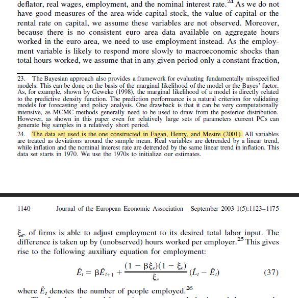
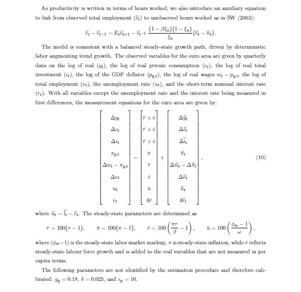
I took this from the paper of Smets, Warne and Wouters (2014). Their equation is based on Smets and Wouters (2003) and they included it to respond to the slower reaction of total employment to exogenous shocks in comparison to hours worked.
Maybe I try to use the auxiliary equation e - e(-1) only as a measurment equation for the difference of observed employment.
Best regards
Did you simply append that equation to your model? Because I presume that is must somehow be integrated into your model.
What do you exactly mean by integrating into my model? That I have to rewrite some of my equations in terms of the new variable e (observed total employment)?
Up to now I just added the equation and the variable to my model.
Yes, that is what I mean. Why otherwise should a pure measurement equation contain expectations of the future?
Yes you are right, that sounds strange and the paper isn‘t very transparent there. But it looks as if the difference of e and e(-1) + its steady state is set just equal to the log difference of observed total employment in the measurment equation and hence it includes the expectation value.
I will further try my luck and keep you in The loop. Thanks for your help!
Have you looked at the original paper they took this feature from?
Yes in Smets/Wouters (2003), they also used the expectation term for their auxiliary observed total employment.
I’ve attached 2 pictures from both papers, in which they explain the equations
There is something weird in the new paper. There is no discounting and and the order in the bracket is switched.
Hi,
I’m wondering where the equation for observed employment is coming from. I see that most of the papers in the literature refer to Smet and Wouters (2003), but they do not explain the micro foundation behind it explicitly. Is there a way to derive the first order condition associated with it?
Thanks in advance!
It seems the equation in the Smets, Warne and Wouters (2014) is the correct one, while the Smets and Wouters (2003) version is misrepresented in the paper. I was able to obtain an old comment by one of the authors that
Eq(37) in the paper is incorrect and deviates from the estimated version. This equation should reflect a Calvo kind of mechanism for employment adjustment and should therefore be specified in terms of E(t)-E(t-1) instead of in terms of E(t).
That explains the version in the 2014 paper, which corresponds to the replication files contained in the Macro Model Database. Note however, that the additional difference of the equation (37) compared to the code and and the 2014 paper is setting \beta=1 in that equation. I guess this makes sense if one thinks of a Calvo type adjustment for employment where no discounting of the future should happen.