Hi all,
I am an undergrad spending my summer learning how to solve rational expectations models and I am trying to learn how to use Dynare. I want to make some IRF’s based on Leeper (1991). The paper is basically about the interaction between monetary and fiscal policy. My only experience with Dynare is from reading Eric Sims’ lecture notes (https://www3.nd.edu/~esims1/using_dynare.pdf).
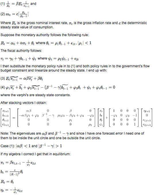
Somehow I managed to solve the model and obtain similar results to Leeper. However, my problem is that I don’t know what equations to include in the model block. I posted this question on EconomicsStackExchange. Here are the key parts:
(1) and (2) are the consumer’s FOC’s and the last 4 equations are the equilibrium solutions.
In Sims’ notes, he derives FOC’s from a basic RBC economy and writes them in the model block. While I only have inflation as a function of shocks. So I am very confused as to what should be included.
I haven’t learned how to solve ratex models in university yet so everything I know is from reading online notes. I do apologise if my questions are too naive.
That very much depends on the setup you want to consider, i.e. whether you want to work with the nonlinear version and let Dynare do the linearization or whether you want to work with the linear version. The latter seems to be easier. In that case, you need equations (3) and (4) (Euler equation and budget constraint) that determine inflation \pi_t and b_t given the two exogenous processes \theta_t and \psi_t and the two AR-processes for these exogenous processes. Basically, you need to implement the stacked system you provided above, but using Dynare’s stock at the end of period notation. Compared to equation (4), you shifted bonds by one period. Also note that the exogenous AR-processes are entered contemporaneously, not in expectations, i.e. use
\theta_t=\rho_1 \theta_{t-1}+\epsilon_{1t}
If you want the full version before substituting out for R_t and m_t, take the linearized versions of (1) and (2) and the budget constraint, plus the two policy rules and the two exogenous processes.
Thank you very much Professor Pfeifer, I really appreciate you taking your time. I followed what you said and finally obtained an IRF! I think my calibration is very poor so the graphs are looking quite strange but at least I now know what to do. Just a couple of thoughts: If I want to include, say, money growth in the IRF, can I define h_{t} = M_{t}/M_{t-1} = m_{t} \pi_{t}/m_{t-1} re-arrange and substitute the equilibrium condition for real balances, linearize and add it to the model block?
Also, the varphi’s in the model consist of steady state values. Right now I calculated each one of them by hand but is it possible to have formulas in the parameter block? For instance can I have: \varphi_{1} = \frac{c}{R -1} = [\frac{1}{\beta \pi} +...] where the variables are calibrated to their steady state values that I define.
One thing regarding Dynare’s end of period notation. In this case B_t represents bond holdings at the beginning of period t (i.e B_t is predetermined in period t). Does this mean equation (4) should include b(-1) and b(-2)?
Thank you once again.
Thank you once again professor. Regarding the 2nd point, I think I’ve understood correctly but I just want to make sure. For example:
parameters alpha, b, beta, gamma, c, R, b, rho1, rho2;
alpha = 1.5; beta = 0.99; c = 7; R = 1.04; rho1 = 0.7; rho2 = 0.7; b = 2;
model; #v1 = (c/R-1)*((1/beta) -(alpha/(R-1))) + (b/beta)
And then similar expressions for v2,v3,v4 and the ‘regular’ variables.
Yes, you will need model-local variables for the composite parameters like the \varphi_i. I am not sure what you mean with
As regular variables like \pi_t are variables, not parameters, you need to define them as var.
Sorry for the confusion, my English isn’t too great. By regular variables I meant everything indexed by time, I just didn’t want to write out the entire code. I understand what needs to be done now though. Many thanks for the help, it is greatly appreciated.
Don’t know if I should start a new post for further questions but it is in relation to the one posted above so I’ll continue this thread. I think I have the basic model under control but I am very confused when I add m_{t}. I think it might be because I am linearising incorrectly. This is what I have done:
From the FOC (eq. (2)) we have m_{t} = c[\frac{R_{t}}{R_{t} - 1}], I then log both sides and do a Taylor approximation around the steady state (denoted by an asterix):
\ln m^* + \frac{1}{m^*}(m_{t} - m^*) = \ln( c[\frac{R^*}{R^* - 1}]) + \frac{1}{ c[\frac{R^*}{R^* - 1}]}(-1)c[\frac{1}{(R^*-1)^2}](R_{t}- R^*)
After some simplification I get \tilde{m} = - \tilde{R_{t}} \frac{1}{R-1}, here the tilde represents deviation from the steady state (i.e \tilde{m} = \frac{m_{t} - m^*}{m^*}. I then include the above in the model block and include the interest rate rule that the central bank follows.
But when I run the simulation, m_{t} does not show up in the IRF.
Also, when I do what Prof. Pfeifer said and include m = R - R(-1) I get the same problem. (But why are our linearisations different?)
And lastly, say I want to include interest rates in the IRF. Could I simply linearise eq. (1), i.e R = pi(+1)?
EDIT: Now I’m even more confused. I added the equation for money growth, h_{t} = M_{t}/M_{t-1} following Prof. Pfeifer’s linearisation along with the linearised version of m_{t} as a function of R_{t} and now h_{t} shows up in the IRF but m_{t} does not. And on top of that, the IRF for h_{t} looks to be identical when I use my linearisation of m_{t} and when I use Prof. Pfeifer’s. It feels like I am missing something quite fundamental because I don’t understand why some variables show up in the IRF while others don’t.
I would need the file. But your linearization is wrong. You did not consider correctly that R_{t-1} is a separate variable for which you have to do a Taylor approximation as well.
Thank you for the reply. I will email the file if that is fine by you. Regarding the linearisation: I think the picture I provided in my OP is poor as it makes it look like R_{t-1}, the correct form is R_{t}-1. In that case my linearisation should be fine, correct?
I see. My mistake. Then your linearization should be fine. Email or PM is fine.
Your linearized condition for m_t tells you that it only depends on R_t, but R_t is constant after a shock to \epsilon_1. In contrast, h depends on inflation as well.
Ah, of course! I understand now. I will try to figure out how to deal with the present value variables over the weekend. I suppose instead of discounting up to infinity I can stop around t = 50 or so.
Thanks once again for all the help 
Yes, that should work. Use the macro-processor for doing the sum.